Expressing an Indicator in Neural Net Form

Recently I started investigating relative rotation graphs with a view to perhaps implementing a version of this for use on forex currency pairs. The underlying idea of a relative rotation graph is to plot an asset's relative strength compared to a benchmark and the momentum of this relative strength and to plot this in a form similar to a Polar coordinate system plot, which rotates around a zero point representing zero relative strength and zero relative strength momentum. After some thought it occurred to me that rather than using relative strength against a benchmark I could use the underlying relative strengths of the individual currencies, as calculated by my currency strength indicator, against each other. Furthermore, these underlying log changes in the individual currencies can be normalised using the ideas of brownian motion and then averaged together over different look back periods to create a unique indicator.

This indicator was coded up in the "traditional" way that will be familiar to anybody who has ever tried coding a trading indicator in any coding language. However, I thought that if the calculation of this indicator could be expressed in the form of a Feedforward neural network then the optimisation opportunities available using backpropagation and regularization could be used to tweek the indicator in more useful ways than just varying a look back length and amount of averaging. After some work I was able to make this work in just these two lines of Octave code:

indicator_middle_layer = tanh( full_feature_matrix * input_weights ) ;
indicator_nn_output = tanh( indicator_middle_layer * output_weights ) ; 

Of course, prior to calling these two lines of code, there is some feature engineering to create the input full_feature_matrix, and the input weights and output_weights matrices taken together are mathematically equivalent to the original indicator calculations. Finally, because this is a neural net expression of the indicator, the non-linear tanh activation function is applied to the hidden middle and output layers of the net.

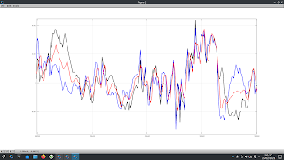
The following plot shows the original indicator in black and the neural net version of it in blue 

over the data shown in this plot of 10 minute bars of the EURUSD forex pair. 

The red indicator in the plot above is the 1 bar momentum of the neural net indicator plot.

To judge the quality of this indicator I used the entropy measure (measured over 14,000+ 10 minute bars of EURUSD), the results of which are shown next.

entropy_indicator_original = 0.9485
entropy_indicator_nn_output = 0.9933

An entropy reading of 0.9933 is probably as good as any trading indicator could hope to achieve (a perfect reading is 1.0) and so the next thing was to quickly back test the indicator performance. Based on the logic of the indicator the obvious long (short) signals are being above (below) the zeroline, or equivalently the sign of the indicator, and for good measure I also tested the sign of the momentum and some simple moving averages thereof.

The following plot shows the equity curves of this quick test where it is visually clear that the blue equity curves are "the best" when plotted in relation to the black "buy and hold" equivalent equity curve. These represent the equity curves of a 3 bar simple moving average of the 1 bar momentum of both the original formulation of the indicator and the neural net implementation. I would point out that these equity curves represent the theoretical equity resulting from trading the London session after 9:00am BST and stopping at 7:00am EST (usually about noon BST) and then starting trading again at 9:00am EST until 17:00pm EST. This schedule avoids the opening sessions (7:00 to 9:00am) in both London and New York because, from my observations of many OHLC charts such as shown above, there are frequently wild swings where price is being pushed to significant points such as volume profile clusters, accumulations of buy/sell orders etc. and in my opinion no indicator can be expected to perform well in that sort of environment. Also avoided are the hours prior to 7:00am BST, i.e. the Asian session or overnight session.    

Although these equity curves might not, at first glance, be that impressive, especially as they do not account for trading costs etc. my intent on doing these tests was to determine the configuration of a final "decision" output layer to be added to the neural net implementation of the indicator. A 3 bar simple moving average of the 1 bar momentum implies the necessity to include 4 consecutive readings of the indicator output as input to a final " decision" layer. The following simple, hand-drawn sketch shows what I mean:

A discussion of this will be the subject of my next post.

A Replacement for my PositionBook Charts using Tick Volumes?

At the end of my previous post I said that I would be looking into using tick volume to create a new indicator, and this post is about the work I have done on this idea.

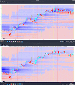
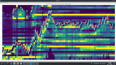
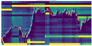
At first I tried creating a more traditional type of indicator using tick volumes separated out into buy and sell volumes, but I quickly felt that this was not a useful investment of my time so I gave up on this idea. Instead, I have come up with a way to plot tick volume levels that are similar to my previously discussed positionbook chart type, which I was forced to give up on because Oanda have discontinued the API endpoint for downloading the required data. An example of the the new, tick volume equivalent is shown below, followed by a brief description of the methodology used to create it.

Starting with the basics, if we imagine a Doji bar, for every up (down) tick there must be a corresponding and opposing down (up) tick for the bar to open and close at the exact same price and therefore we can split the tick volume for the bar equally between buy and sell tick volumes. Similarly, if we imagine a bar that opens on the low (high) and closes on the high (low), the number of ticks within the entire bar tick range can be ascribed to buy (sell) volume and the balance divided between buy and sell.

e.g. a bar opens at the low , closes at the high, with a tick range of 10 and total tick volume of 50 then:

• buy tick volume = 10 + ( 50 - 10)/2 = 30
• sell tick volume = 50 - buy tick volume = 20

This idea can be generalised to the range of a candlestick body being appropriately allocated to buy or sell tick volume, with the remaining balance of the total bar volume being equally allocated to buy and sell. OK, so far so good, and nothing particularly ground breaking. For the want of explaining it in a more precise manner, using the "geometry" of a bar to allocate buy and sell volumes is something that can be found online in the formulation of more than a few indicators.

The next step step is to "smear" these buy and sell volumes equally across the whole range of the bar and then take the difference:

e.g. "smeared" buy - "smeared" sell = 30 / 10 - 20 / 10 = 1, thus allocate a tick difference value of +1 for each tick level within the 10 tick range of the bar. 

Of course, over a large (e.g. 10 minute bar) this wouldn't necessarily be very informative as it is known (my volume profile bars) that the volume is usually unevenly spread across the range of any given bar. The solution to this is to apply the above methodology to the smallest bar possible, and with Oanda the smallest possible bar download is a 5 second bar. Thus what I have done is apply the above to each 5 second bar within a given 10 minute bar period and then accumulate the buy/sell/tick difference values across the individual tick levels within the 10 minute bar. This gives tick differences values that approximate the differences between each bar's separate buy and sell volume profiles.

The final step is to volume normalise the above calculations by using the total 10 minute bar tick volume such that tick differences within bars that have higher total tick volume have a greater weight than those in low tick volume bars. This is simply done by setting the total bar volume as the numerator and the tick difference as the denominator:

e.g. a tick difference of 2 at a tick level within a bar with a total 10 tick volume will get the weight

•  10 / 2 = 5

whilst the same tick difference in a 50 tick volume bar will get the weight

• 50 / 2 = 25

Finally, all the above is plotted as the backgound heatmap to a candlestick chart, but with a slight twist - exponential forgetting is applied along each individual tick level within the y-axis range such that if an individual tick level only has one price bar spanning it the colour slowly fades as we move along the x-axis, whilst if this level is revisited, just as with an exponential moving average, the more recent data is accumulatively weighted more. For the above plot the exponential alpha value is set at the equivalent of a 144 bar exponential moving average, i.e. the number of 10 minute bars in a 24 hour period. Shorter moving average equivalents just increase the speed at which the forgetting takes place, leading to shorter lines extending to the right, but accentuate the differences between levels; e.g. the following is the same plot as above with the equivalent of a 14 bar exponential moving average alpha value.

Earlier in this post I alluded to the possibility of this type of tick difference chart being a replacement for my unwillingly and forcefully retired PositionBook chart type. The similarities/equivalences between the two chart types I now discuss:

With the old PositionBook (PB) chart, traders' net positions at any given level and at 20 minute snapshot frequency were explicitly given by API data download and changes between snapshots were inferred by an optimisation routine. With these new TickDifference (TD) charts, traders' net positions are inferred via the methodology described above, i.e. higher normalised tick volumes at different tick levels imply a higher, net trader positioning at these levels, and changes over time in this positioning are approximated by the exponential forgetting factor.

In terms of plotting, both in the PB and TD charts, the intensities of the colours (blue for longs and red for shorts) reflect the relative importances of long/short positioning at different levels: the greater the intensity, the greater the difference between long and short positioning.

I shall now enter into a period of observational study of the usefulness of this chart type because, as the chart is inherently visual, I can't imagine how I could effectively test it in a more traditional, back testing manner. If any reader could suggest how this more traditional approach might be done, I'm all ears.    

 

Use of HDF5 Format, and Some Charting Improvements

Over the last few weeks/months I have found it necessary to revisit the basic infrastructure of my trading/computing set up due to increasing slowness of the various computing routines I have running.

The first issue I am now addressing is how I store my data on disc. When I first started I opted for csv text files, mostly due to my ignorance of other possibilities at the time and the fact that I could visually inspect the files to manually check things. However, for my data retrieval and use needs this is now becoming too slow and burdensome and so I have made the decision to switch over to the HDF5 format and use the hdf5oct package for Octave for my data storage and file I/O needs. This dramatically speeds up data loading and will enable me to consolidate my disparate csv text files into individual tradable instrument HDF5 files, where all the data for the said tradable instrument is contained in a single HDF5 file. This data migration is an ongoing process that will continue for a few months, with the associated changes in my workflow, rewriting of some scripts and functions, cronjobs, etc.

The next thing I have done is slightly improved the calculation methodology and plotting of my volume profile bars, and the following chart shows the new version volume profile bars for the last three, 10 minute bars on the EUR-USD forex pair for trading on Friday, 4th April 2025,

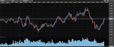
whilst this second chart shows the equivalent time period with 5 second OHLC candles and the associated tick volumes for each bar.

 

The vertical green lines on this second chart delineate the 5 second bars into the corresponding 10 minute bars in the first chart. I think it is quite easy to visually see the correspondence between the 10 minute volume profile bars and the 5 second OHLC bars. 

Another thing I also plan to do in the forthcoming weeks is to use the tick volume (as shown in the second chart above) to create a new type of indicator, but more on that in due course.

A "New" Way to Smooth Price

Below is code for an Octave compiled C++ .oct function to smooth price data.

#include "octave oct.h"
#include "octave dcolvector.h"
#include "octave dmatrix.h"
#include "GenFact.h"
#include "GramPoly.h"
#include "Weight.h"

DEFUN_DLD ( double_smooth_proj_2_5, args, nargout,
"-*- texinfo -*-\n\
@deftypefn {Function File} {} double_smooth_proj_2_5 (@var{input_vector})\n\
This function takes an input series and smooths it by projecting a 5 bar rolling linear fit\n\
3 bars into the future and using these 3 bars plus the last 3 bars of the rolling input\n\
to fit a FIR filter with a 2.5 bar lag from the last projected point, i.e. a 0.5 bar\n\
lead over the last actual rolling point in the series. This is averaged with the previously\n\
calculated such smoothed point for a theoretical zero-lagged smooth. This smooth is\n\
again smoothed as above for a smooth of the smooth, i.e. a double-smooth of the\n\
original input series. The double_smooth and smooth are the function outputs.\n\
@end deftypefn" )

{
octave_value_list retval_list ;
int nargin = args.length () ;

// check the input arguments
if ( nargin > 1 ) // there must be a single, input price vector
   {
   error ("Invalid arguments. Inputs are a single, input price vector.") ;
   return retval_list ;
   }

if ( args(0).length () < 5 )
   {
   error ("Invalid 1st argument length. Input is a price vector of length >= 5.") ;
   return retval_list ;
   }
// end of input checking

ColumnVector input = args(0).column_vector_value () ;
ColumnVector smooth = args(0).column_vector_value () ;
ColumnVector double_smooth = args(0).column_vector_value () ;

// create the fit coefficients matrix
int p = 5 ;             // the number of points in calculations
int m = ( p - 1 ) / 2 ; // value to be passed to call_GenPoly_routine_from_octfile
int n = 1 ;             // value to be passed to call_GenPoly_routine_from_octfile
int s = 0 ;             // value to be passed to call_GenPoly_routine_from_octfile

  // create matrix for fit coefficients
  Matrix fit_coefficients_matrix ( 2 * m + 1 , 2 * m + 1 ) ;
  // and assign values in loop using the Weight.h recursive Gram Polynomial C++ headers
  for ( int tt = -m ; tt < (m+1) ; tt ++ )
  {
        for ( int ii = -m ; ii < (m+1) ; ii ++ )
        {
        fit_coefficients_matrix ( ii + m , tt + m ) = Weight( ii , tt , m , n , s ) ;
        }
  }

  // create matrix for slope coefficients
  Matrix slope_coefficients_matrix ( 2 * m + 1 , 2 * m + 1 ) ;
  s = 1 ;
  // and assign values in loop using the Weight.h recursive Gram Polynomial C++ headers
  for ( int tt = -m ; tt < (m+1) ; tt ++ )
  {
        for ( int ii = -m ; ii < (m+1) ; ii ++ )
        {
        slope_coefficients_matrix ( ii + m , tt + m ) = Weight( ii , tt , m , n , s ) ;
        }
  }

  Matrix smooth_coefficients ( 1 , 5 ) ;
  // fill the smooth_coefficients matrix, smooth_coeffs = ( 9/24 ) .* fit_coeffs + ( 7/12 ) .* slope_coeffs + [ 0 ; 1/24 ; 1/8 ; 5/24 ; 1/4 ] ;
  smooth_coefficients( 0 , 0 ) = ( 9.0 / 24.0 ) * fit_coefficients_matrix( 0 , 4 ) + ( 7.0 / 12.0 ) * slope_coefficients_matrix( 0 , 4 ) ;
  smooth_coefficients( 0 , 1 ) = ( 9.0 / 24.0 ) * fit_coefficients_matrix( 1 , 4 ) + ( 7.0 / 12.0 ) * slope_coefficients_matrix( 1 , 4 ) + ( 1.0 / 24.0 ) ;
  smooth_coefficients( 0 , 2 ) = ( 9.0 / 24.0 ) * fit_coefficients_matrix( 2 , 4 ) + ( 7.0 / 12.0 ) * slope_coefficients_matrix( 2 , 4 ) + ( 1.0 / 8.0 ) ;
  smooth_coefficients( 0 , 3 ) = ( 9.0 / 24.0 ) * fit_coefficients_matrix( 3 , 4 ) + ( 7.0 / 12.0 ) * slope_coefficients_matrix( 3 , 4 ) + ( 5.0 / 24.0 ) ;
  smooth_coefficients( 0 , 4 ) = ( 9.0 / 24.0 ) * fit_coefficients_matrix( 4 , 4 ) + ( 7.0 / 12.0 ) * slope_coefficients_matrix( 4 , 4 ) + ( 1.0 / 4.0 ) ;

    for ( octave_idx_type ii (4) ; ii < args(0).length () ; ii++ )
        {

         smooth( ii ) = smooth_coefficients( 0 , 0 ) * input( ii - 4 ) + smooth_coefficients( 0 , 1 ) * input( ii - 3 ) + smooth_coefficients( 0 , 2 ) * input( ii - 2 ) +
                        smooth_coefficients( 0 , 3 ) * input( ii - 1 ) + smooth_coefficients( 0 , 4 ) * input( ii ) ;

         double_smooth( ii ) = smooth_coefficients( 0 , 0 ) * smooth( ii - 4 ) + smooth_coefficients( 0 , 1 ) * smooth( ii - 3 ) + smooth_coefficients( 0 , 2 ) * smooth( ii - 2 ) +
                               smooth_coefficients( 0 , 3 ) * smooth( ii - 1 ) + smooth_coefficients( 0 , 4 ) * smooth( ii ) ;

        }

retval_list( 0 ) = double_smooth ;
retval_list( 1 ) = smooth ;

return retval_list ;

} // end of function

Rather than describe it, I'll just paste the "help" description below:-

"This function takes an input series and smooths it by projecting a 5 bar rolling linear fit 3 bars into the future and using these 3 bars plus the last 3 bars of the rolling input to fit a FIR filter with a 2.5 bar lag from the last projected point, i.e.  a 0.5 bar lead over the last actual rolling point in the series.  This is averaged with the previously calculated such smoothed point for a theoretical zero-lagged smooth.  This smooth is again smoothed as above for a smooth of the smooth, i.e.  a double-smooth of the original input series.  The double_smooth and smooth are the function outputs."

The above function calls previous code of mine to calculate savitzky golay filter convolution coefficients for internal calculations, but for the benefit of readers I will simply post the final coefficients for a 5 tap FIR filter.

-0.191667  -0.016667   0.200000   0.416667   0.591667

These coefficients are for a "single" smooth. Run the output from a function using these through the same function to get the "double" smooth.

Testing on a sinewave looks like this:-

where the cyan, green and blue filters are the original FIR filter with 2.5 bar lag, a 5 bar SMA and Ehler's super smooth (see code here) applied to sinewave "price" for comparative purposes. The red filter is my "double_smooth" and the magenta is a Jurik Moving Average using an Octave adaptation of code that is/was freely available on the Tradingview website. The parameters for this Jurik average (length, phase and power) were chosen to match, as closely as possible, those of the double_smooth for an apples to apples comparison.

I will not discuss this any further in this post other than to say I intend to combine this with the ideas contained in my new use for kalman filter post.

More in due course.

Downloading Dukascopy Tick Data with Node Library

As part of my investigations into forex news trading I have found it necessary to obtain forex tick level data for back testing purposes and below I provide code to achieve this using Dukascopy's Node library, being called from Octave and using some system calls. A useful youtube video about the Dukascopy Node library will give readers some background information.

function [ first_days , last_days ] = first_and_last_weekday_of_month( y )
  t1 = datenum( [ y , 1 , 1 , 0 , 0 , 0 ] ) ;
  t2 = datenum( [ y , 12 , 31 , 0 , 0 , 0 ] ) ;
  t  = datevec( t1 : t2 ) ;
  delete_ix = strcmp( 'Saturday' , datestr( t , 'dddd' ) ) ; % find all Saturdays
  t( delete_ix , : ) = [] ;
  delete_ix = strcmp( 'Sunday' , datestr( t , 'dddd' ) ) ; % find all Sundays
  t( delete_ix , : ) = [] ;
  first_day_ix = find( diff( [ 1 ; t( : , 2 ) ] ) > 0 ) ;
  first_days = [ t( 1 , : ) ; t( first_day_ix , : ) ] ;
  last_day_ix = first_day_ix - 1 ; last_day_ix( last_day_ix <= 0 ) = [] ;
  last_days = [ t( last_day_ix , : ) ; t( end , : ) ] ;
endfunction

ii_vec = [ 2020 , 2021 , 2022 , 2023 , 2024 ] ;

for ii = ii_vec

[ first_days , last_days ] = first_and_last_weekday_of_month( ii ) ;

  for jj = 1 : 12
  cd /path/to/folder ;
  command = [ 'npx dukascopy-node -i eurusd -from ' , datestr( first_days( jj , : ) , 29 ) , ' -to ' , datestr( last_days( jj , : ) , 29 ) , ...
               ' --timeframe tick --format csv --retries 5 --directory eurusd --date-format "YYYY-MM-DD HH:mm:ss:SSS" ' ] ;
  system( command ) ;

  cd /path/to/folder/eurusd ;

  ## delete header
  command = [ "sed -i '/timestamp,askPrice,bidPrice/d' eurusd-tick-" , datestr( first_days( jj , : ) , 29 ) , "-" , datestr( last_days( jj , : ) , 29 ) , ".csv" ] ;
  system( command ) ;

  FID = fopen( 'eurusd-tick-2015-10-02-2015-10-03.csv' , 'r' ) ;
  FID = fopen( [ 'eurusd-tick-' , datestr( first_days( jj , : ) , 29 ) , '-' , datestr( last_days( jj , : ) , 29 ) , '.csv' ] , 'r' ) ;
  sizeM = [ 9 , Inf ] ;
  M = fscanf( FID , "%4d-%2d-%2d %2d:%2d:%2d:%3d,%f,%f" , sizeM )' ;
  fclose( FID ) ;

  save( '-binary' , [ 'eurusd-' , num2str( ii ) , '-' , num2str( first_days( jj , 2 ) ) , '.bin' ] , 'M' ) ;
  delete( 'eurusd-tick-*' ) ;

  clear -x ii_vec ii jj first_days last_days first_and_last_weekday_of_month

  endfor ## jj loop

clear -x ii_vec ii first_and_last_weekday_of_month

endfor ## ii_vec

The result of running the above code results in a folder full of tick data saved in Octave's native binary format, one file per month, with each file's name being descriptive of the data contained within.

I hope readers will find this useful.

Using Oanda's API to Place Entry Orders

Since my last post about end of initial testing I have been working on Oanda API functions in Octave to programmatically place entry orders and associated take profit and stop orders for a future possible forex news trading system. The reason for this is simple - it would be next to impossible to manually place a series of entry orders in the last few moments before a news release, so this would have to be done automatically. To this end, I have spent the last few weeks writing a few simple entry functions and testing them in my live trading account with the minimum trading size, i.e. buying and selling 1 Euro in the EURUSD forex pair and observing the subsequent lines at the entry/stop/take profit levels that appear on the live web platform.

The basic schema for this is shown in the following code box, where it can be seen that

body = jsonencode( struct( 'order' , struct( 'units' , num2str( 1 ) , ...
                                              'instrument' , 'EUR_USD' , ...
                                              'timeInForce' , 'FOK' , ...
                                              'type' , 'MARKET' , ...
                                              'trailingStopLossOnFill' , struct( 'distance' , num2str( trail_distance ) , ...
                                                                                  'timeInForce' , 'GTC' , ...
                                                                                  'triggerCondition' , 'MID' ) , ...
                                              'positionFill' , 'DEFAULT' ) ) )

account_header = ['curl -X POST -H "Content-Type: application/json" -H "Authorization: Bearer TOKEN"'] ;

submit_order = [ account_header , ' "https://api-fxtrade.oanda.com/v3/accounts/ACCOUNT/orders"' , ' -d ' , "'" , body , "'" ] ;

[ ~ , ret_JSON ] = system( submit_order , RETURN_OUTPUT = 'TRUE' ) ;

a JSON object containing the order details is created, HTML headers with account information are added, and then the order is dispatched via a system call to the cURL library.

A more complete Octave function example is shown next. This is a buy on a stop entry function which also sets a stop loss and take profit target level on being filled, and there is also some basic input checking.

function [ ret_JSON ] = buy_stop_entry_with_stoploss_and_takeprofit( cross , no_of_units , entry_price_level , stop_level , take_profit_level )

## some basic checks
if ( entry_price_level <= stop_level )
   error( 'Stop Level is not below Entry Level.' ) ;
endif

if ( entry_price_level >= take_profit_level )
   error( 'Take Profit Level is not above Entry Level.' ) ;
endif

account_header = ['curl -X POST -H "Content-Type: application/json" -H "Authorization: Bearer TOKEN"'] ;

body = jsonencode( struct( 'order' , struct( 'type' , 'STOP' , ...
                                              'instrument' , toupper( cross ) , ...
                                              'units' , num2str( abs( no_of_units ) ) , ...
                                              'price' , num2str( entry_price_level ) , ...
                                              'stopLossOnFill' , struct( 'price' , num2str( stop_level ) , ...
                                                                         'timeInForce' , 'GTC' ) , ...
                                              'takeProfitOnFill' , struct( 'price' , num2str( take_profit_level ) ) , ...
                                              'timeInForce' , 'GTC' , ...
                                              'triggerCondition' , 'MID' , ...
                                              'positionFill' , 'DEFAULT' ) ) ) ;

submit_order = [ account_header , ' -d ' , "'" , body , "'" , ' "https://api-fxtrade.oanda.com/v3/accounts/ACCOUNT/orders"' ] ;

[ ~ , ret_JSON ] = system( submit_order , RETURN_OUTPUT = 'TRUE' ) ;

ret_JSON = jsondecode( ret_JSON ) ;

endfunction

I won't spend much time explaining the contents of the JSON body as readers can find more information about this in Oanda's online documentation, however, there is one important thing I would note here and that is the key/value pair

 'triggerCondition' , 'MID'

The 'default' value for this is the bid/ask price for sells/buys which, in the case of a news trading system, could be problematic because the spread may very well be widened prior to a news release and trigger an entry without the underlying price actually having moved to the entry level, or even before the news is released. By setting the trigger condition to 'MID' a trade will be entered when the mid-price hits the entry level. The trade-off in this choice is summarised thus:

• if the 'default' value is used, entries on "good" trades will be much closer to the entry level, on average, but at the possible expense of far more false entries and therefore losing trades, versus:
• if the 'MID' value is used, there will possibly be fewer false entries, but at the expense of a worse entry price for "good" trades.

 This is a trade-off that will have to be investigated/tested in due course.

A "New" Use for Kalman Filter on Price Time Series?

During the course of writing this blog I have visited the idea of using Kalman filters several times, most recently in this February 2023 post. My motivation in these previous posts could best be described as trying to smooth price data with as little lag as possible, i.e. create a zero-lag indicator. In doing so, the model most often used for the Kalman filter was a physical motion model with position, velocity and acceleration components. Whilst these "worked" in the sense of smoothing the underlying data, it is not necessarily a good model to use on financial data because, obviously, financial data is not a physical system and so I thought I would apply the Kalman filter to something that is ubiquitously used on financial data - the Exponential moving average.

Below is an Octave function to calculate a "Kalman_ema" where the prediction part of the filter is just a linear extrapolation of an exponential moving average and then this extrapolated value is used to calculate the projected price, with the measurement being the real price and its ema value.

## Copyright (C) 2024 dekalog
##
## This program is free software: you can redistribute it and/or modify
## it under the terms of the GNU General Public License as published by
## the Free Software Foundation, either version 3 of the License, or
## (at your option) any later version.
##
## This program is distributed in the hope that it will be useful,
## but WITHOUT ANY WARRANTY; without even the implied warranty of
## MERCHANTABILITY or FITNESS FOR A PARTICULAR PURPOSE.  See the
## GNU General Public License for more details.
##
## You should have received a copy of the GNU General Public License
## along with this program.  If not, see .

## -*- texinfo -*-
## @deftypefn {} {@var{retval} =} kalman_ema (@var{price}, @var{lookback})
##
## @seealso{}
## @end deftypefn

## Author: dekalog 
## Created: 2024-04-08

function [ filter_out , P_out ] = kalman_ema ( price , lookback )

## check price is row vector
if ( size( price , 1 ) > 1 && size( price , 2 ) == 1 )
 price = price' ;
endif

P_out = zeros( numel( price ) , 2 ) ;

ema_price = ema( price , lookback )' ;
alpha = 2 / ( lookback + 1 ) ;

## initial covariance matrix
P = eye( 3 ) ;

## transistion matrix
A = [ 0 , ( 1 + alpha ) / alpha , -( 1 / alpha ) ; ...
       0 , 2 , -1 ; ...
       0 , 1 , 0 ] ;

## initial Q
Q = eye( 3 ) ;

## measurement vector
Y = [ price ; ...
       ema_price ; ...
       shift( ema_price , 1 ) ] ;
Y( 3 , 1 ) = Y( 2 , 1 ) ;

## measurement matrix
H = eye( 3 ) ;

## measurement noise covariance
R = eye( 3 ) ;

## container for Kalman filter output
filter_out = zeros( size( Y ) ) ;
errors = ones( 3 , 1 ) ;

for ii = 2 : size( Y , 2 )

  X = A * filter_out( : , ii - 1 ) ;
  P = A * P * A' + Q ;

  errors = alpha .* abs( X - Y( : , ii ) ) + ( 1 - alpha ) .* errors ;

  IM = H * X ; ## Mean of predictive distribution
  IS = ( R + H * P * H' ) ; ## Covariance of predictive mean
  K = P * H' / IS ; ## Computed Kalman gain
  X = X + K * ( Y( : , ii ) - IM ) ; ## Updated state mean
  P = P - K * IS * K' ; ## Updated state covariance

  filter_out( : , ii ) = X ;
  P_out( ii , 1 ) = P( 1 , 1 ) ;
  P_out( ii , 2 ) = P( 2 , 2 ) ;

  ## update Q and R
  Q( 1 , 1 ) = errors( 1 ) ; Q( 2 , 2 ) = errors( 2 ) ; Q( 3 , 3 ) = errors( 3 ) ;
  R = Q ;

endfor

filter_out = filter_out' ;

endfunction

Using this for smoothing either the price or the ema has no utility, but a by-product of the filter is the Covariance matrix from which it is possible to plot bands around the price series. The following chart shows the bands for various ema alpha values corresponding to various Fibonacci sequence length look backs for the ema alpha value.  

This next chart, for purposes of clarity, shows the "Golden Cross" lengths of 50 and 200

and this final chart shows an adaptive look back length which is a function of the instantaneous measured period (see here or here) of the underlying data.

Despite the wide range of the input look back lengths for the ema, it can be seen that the covariance bands around price are broadly similar. I can think of many uses for such a data driven but basically parameter insensitive measure of price variance, e.g. entry/exit levels, stop levels, position sizing etc.

More in due course.

Judging the Quality of Indicators.

In my previous post I said I was trying to develop new indicators from the results of my new PositionBook optimisation routine. In doing so, I need to have a methodology for judging the quality of the indicator(s). In the past I created a Data-Snooping-Tests-GitHub which contains some tests for statistical significance testing and which, of course, can be used on these new indicators. Additionally, for many years I have had a link to tssb on this blog from where a free testing program, VarScreen, and its associated manual are available. Timothy Masters also has a book, Testing and Tuning Market Trading Systems, wherein there is C++ code for an Entropy test, an Octave compiled .oct version of which is shown in the following code box.

#include "octave oct.h"
#include "octave dcolvector.h"
#include "cmath"
#include "algorithm"

DEFUN_DLD ( entropy, args, nargout,
"-*- texinfo -*-\n\
@deftypefn {Function File} {entropy_value =} entropy (@var{input_vector,nbins})\n\
This function takes an input vector and nbins and calculates\n\
the entropy of the input_vector. This input_vector will usually\n\
be an indicator for which we want the entropy value. This value ranges\n\
from 0 to 1 and a minimum value of 0.5 is recommended. Less than 0.1 is\n\
serious and should be addressed. If nbins is not supplied, a default value\n\
of 20 is used. If the input_vector length is < 50, an error will be thrown.\n\
@end deftypefn" )

{
octave_value_list retval_list ;
int nargin = args.length () ;
int nbins , k ;
double entropy , factor , p , sum ;

// check the input arguments
if ( args(0).length () < 50 )
   {
   error ("Invalid 1st argument length. Input is a vector of length >= 50.") ;
   return retval_list ;
   }

if ( nargin == 1 )
   {
   nbins = 20 ;
   }

if ( nargin == 2 )
   {
   nbins = args(1).int_value() ;
   }
// end of input checking

ColumnVector input = args(0).column_vector_value () ;
ColumnVector count( nbins ) ;
double max_val = *std::max_element( &input(0), &input( args(0).length () - 1 ) ) ;
double min_val = *std::min_element( &input(0), &input( args(0).length () - 1 ) ) ;
factor = ( nbins - 1.e-10 ) / ( max_val - min_val + 1.e-60 ) ;

for ( octave_idx_type ii ( 0 ) ; ii < args(0).length () ; ii++ ) {
      k = ( int ) ( factor * ( input( ii ) - min_val ) ) ;
      ++count( k ) ; }

sum = 0.0 ;
for ( octave_idx_type ii ( 0 ) ; ii < nbins ; ii++ ) {
      if ( count( ii ) ) {
         p = ( double ) count( ii ) / args(0).length () ;
        sum += p * log ( p ) ; }
        }

entropy = -sum / log ( (double) nbins ) ;

retval_list( 0 ) = entropy ;

return retval_list ;

} // end of function

This calculates the information content, Entropy_(information_theory), of any indicator, the value for which ranges from 0 to 1, with a value of 1 being ideal. Masters suggests that a minimum value of 0.5 is acceptable for indicators and also suggests ways in which the calculation of any indicator can be adjusted to improve its entropy value. By way of example, below is a plot of an "ideal" (blue) indicator, which has values uniformly spread across its range

with an entropy value of 0.9998. This second plot shows a "good" indicator, which has an

entropy value of 0.7781 and is in fact just random, normally distributed values with a mean of 0 and variance 1. In both plots, the red indicators fail to meet the recommended minimum value, both having entropy values of 0.2314.

It is visually intuitive that in both plots the blue indicators convey more information than the red ones. In creating my new PositionBook indicators I intend to construct them in such a way as to maximise their entropy before I progress to some of the above mentioned tests.

Update to PositionBook Chart - Revised Optimisation Method

Just over a year ago I previewed a new chart type which I called a "PositionBook Chart" and gave examples in this post and this one. These first examples were based on an optimisation routine over 6 variables using Octave's fminunc function, an unconstrained minimisation routine. However, I was not 100% convinced that the model I was using for the loss/cost function was realistic, and so since the above posts I have been further testing different models to see if I could come up with a more satisfactory model and optimisation routine. The comparison between the original model and the better, newer model I have selected is indicated in the following animated GIF, which shows the last few day's action in the GBPUSD forex pair. 

The old model is figure(200), with the darker blue "blob" of positions accumulated at the lower, beginning of the chart, and the newer model, figure(900), shows accumulation throughout the uptrend. The reasons I prefer this newer model are:

• 4 of the 6 variables mentioned above (longs above and below price bar range, and shorts above and below price bar range) are theoretically linked to each other to preserve their mutual relationships and jointly minimised over a single input to the loss/cost function, which has a bounded upper and lower limit. This means I can use Octave's fminbnd function instead of fminunc. The minimisation objective is the minimum absolute change in positions outside the price bar range, which has a real world relevance as compared to the mean squared error of the fminunc cost function.
• because fminunc is "unconstrained" occasionally it would converge to unrealistic solutions with respect to position changes outside the price bar range. This does not happen with the new routine.
• once the results of fminbnd are obtained, it is possible to mathematically calculate the position changes within the price bar range exactly, without needing to resort to any optimisation routine. This gives a zero error for the change which is arguably the most important.
• the results from the new routine seem to be more stable in that indicators I am trying to create from them are noticeably less erratic and confusing than those created from fminunc results.
• finally, fminbnd over 1 variable is much quicker to converge than fminunc over 6 variables.
  

The second last mentioned point, derived indicators, will be the subject of my next post.

Currency Strength Revisited

Recently I responded to a Quantitative Finance forum question here, where I invited the questioner to peruse certain posts on this blog. Apparently the posts do not provide enough information to fully answer the question (my bad) and therefore this post provides what I think will suffice as a full and complete reply, although perhaps not scientifically rigorous.

The original question asked was "Is it possible to separate or decouple the two currencies in a trading pair?" and I believe what I have previously described as a "currency strength indicator" does precisely this (blog search term ---> https://dekalogblog.blogspot.com/search?q=currency+strength+indicator). This post outlines the rationale behind my approach.

Take, for example, the GBPUSD forex pair, and further give it a current (imaginary) value of 1.2500. What does this mean? Of course it means 1 GBP will currently buy you 1.25 USD, or alternatively 1 USD will buy you 1/1.25 = 0.8 GBP. Now rather than write GBPUSD let's express GBPUSD as a ratio thus:- GBP/USD, which expresses the idea of "how many USD are there in a GBP?" in the same way that 9/3 shows how many 3s there are in 9. Now let's imagine at some time period later there is a new pair value, a lower case "gbp/usd" where we can write the relationship

                    (1)     ( GBP / USD ) * ( G / U ) = gbp / usd

to show the change over the time period in question. The ( G / U ) term is a multiplicative term to show the change in value from old GBP/USD 1.2500 to say new value gbp/usd of 1.2600, 

e.g.                ( G / U ) == ( gbp / usd ) / ( GBP / USD ) == 1.26 / 1.25 == 1.008

from which it is clear that the forex pair has increased by 0.8% in value over this time period. Now, if we imagine that over this time period the underlying, real value of USD has remained unchanged this is equivalent to setting the value U in ( G / U ) to exactly 1, thereby implying that the 0.8% increase in the forex pair value is entirely attributable to a 0.8% increase in the underlying, real value of GBP, i.e. G == 1.008. Alternatively, we can assume that the value of GBP remains unchanged,

 e.g.                G == 1, which means that U == 1 / 1.008 == 0.9921

which implies that a ( 1 - 0.9921 ) == 0.79% decrease in USD value is responsible for the 0.8% increase in the pair quote.

Of course, given only equation (1) it is impossible to solve for G and U as either can be arbitrarily set to any number greater than zero and then be compensated for by setting the other number such that the constant ( G / U ) will match the required constant to account for the change in the pair value.

However, now let's introduce two other forex pairs (2) and (3) and thus we have:-

                    (1)     ( GBP / USD ) * ( G / U ) = gbp / usd

                    (2)     ( EUR / USD ) * ( E / U ) = eur / usd

                    (3)     ( EUR / GBP ) * ( E / G ) = eur / gbp

We now have three equations and three unknowns, namely G, E and U, and so this system of equations could be laboriously, mathematically solved by substitution. 

However, in my currency strength indicator I have taken a different approach. Instead of solving mathematically I have written an error function which takes as arguments a list of G, E, U, ... etc. for all currency multipliers relevant to all the forex quotes I have access to, approximately 47 various crosses which themselves are inputs to the error function, and this function is supplied to Octave's fminunc function to simultaneously solve for all G, E, U, ... etc. given all forex market quotes. The initial starting values for all G, E, U, ... etc. are 1, implying no change in values across the market. These starting values consistently converge to the same final values for G, E, U, ... etc for each separate period's optimisation iterations.

Having got all G, E, U, ... etc. what can be done? Well, taking G for example, we can write

                    (4)     GBP * G = gbp

for the underlying, real change in the value of GBP. Dividing each side of (4) by GBP and taking logs we get

                    (5)     log( G ) = log( gbp / GBP )

i.e. the log of the fminunc returned value for the multiplicative constant G is the equivalent of the log return of GBP independent of all other currencies, or as the original forum question asked, the (change in) value of GBP separated or decoupled the from the pair in which it is quoted.

Of course, having the individual log returns of separated or decoupled currencies, there are many things that can be done with them, such as:-

• create indices for each currency
• apply technical analysis to these separate indices
• intermarket currency analysis
• input to machine learning (ML) models
• possibly create new and unique currency indicators

Examples of the creation of "alternative price charts" and indices are shown below

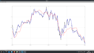
where the black line is the actual 10 minute closing prices of GBPUSD over the last week (13th to 18th August) with the corresponding GBP price (blue line) being the "alternative" GBPUSD chart if U is held at 1 in the ( G / U ) term and G allowed to be its derived, optimised value, and the USD price (red line) being the alternative chart if G is held at 1 and U allowed to be its derived, optimised value.

This second chart shows a more "traditional" index like chart

where the starting values are 1 and both the G and U values take their derived values. As can be seen, over the week there was upwards momentum in both the GBP and USD, with the greater momentum being in the GBP resulting in a higher GBPUSD quote at the end of the week. If, in the second chart the blue GBP line had been flat at a value of 1 all week, the upwards momentum in USD would have resulted in a lower week ending quoted value of GBPUSD, as seen in the red USD line in the first chart. Having access to these real, decoupled returns allows one to see through the given, quoted forex prices in the manner of viewing the market as though through X-ray vision. 

I hope readers find this post enlightening, and if you find some other uses for this idea, I would be interested in hearing how you use it.
 

Quick Update on Kalman Filter and Sensor Fusion

Managed to code it up and get it working, but at the end of the day I couldn't see any value added over just averaging the output of the indicators I was trying to fuse together via Kalman filtering. As a result, I'm giving up on this for now and looking at other things.

More in due course. 

Kalman Filter and Sensor Fusion.

In the Spring of 2012 and again in the Spring of 2019 I posted a series of posts about the Kalman Filter, which readers can access via the blog archive on the right. In both cases I eventually gave up those particular lines of investigation because of disappointing results. This post is the first in a new series about using the Kalman Filter for sensor fusion, which I had known of before, but due to the paucity of clear information about this online I had never really investigated. However, my recent discovery of this Github and its associated online tutorial has inspired me to a third attempt at using Kalman Filters. What I am going to attempt to do is use the idea of sensor fusion to fuse the output of several functions I have coded in the past, which each extract the dominant cycle from a time series, to hopefully obtain a better representation of the "true underlying cycle."

The first step in this process is to determine the measurement noise covariance or, in Kalman Filter terms, the "R" covariance matrix. To do this, I have used the average of two of the outputs from the above mentioned functions to create a new cycle and similarly used two extracted trends (price minus these cycles) averaged to get a new trend. The new cycle and new trend are simply added to each other to create a new price series which is almost identical to the original price series. The screenshot below shows a typical cycle extract,

where the red cycle is the average of the other two extracted cycles, and this following screenshot shows the new trend in red plus the new price alongside the old price (blue and black respectively).

Having created a time series thus with known trend and cycle, it is a simple matter to run my cycle extractor functions on this new price, compare the outputs with the known cyclic component of price and calculate the variance of the errors to get the R covariance matrices for 14 different currency crosses.

More in due course.

 

PositionBook Chart Example Trade

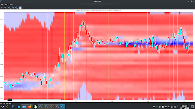
As a quick follow up to my previous post I thought I'd show an example of how one could possibly use my new PositionBook chart as a trade set-up. Below is the USD_CHF forex pair for the last two days

showing the nice run-up yesterday and then the narrow range of Friday's Asian session.

The tentative set-up idea is to look for such a narrow range and use the colour of the PositionBook chart in this range (blue for a long) to catch or anticipate a breakout. The take profit target would be the resistance suggested by the horizontal yellow bar in the open orders chart (overhead sell orders) more or less at Thursday's high.

I decided to take a really small punt on this idea but took a small loss of 0.0046 GBP

as indicated in the above Oanda trade app. I entered too soon and perhaps should have waited for confirmation (I can see a doji bar on the 5 minute chart just after my stop out) or had the conviction to re-enter the trade after this doji bar. The initial trade idea seems to have been sound as the profit target was eventually hit. This could have been a nice 4/5/6 R-multiple profitable trade.😞

Simple Machine Learning Models on OrderBook/PositionBook Features

This post is about using OrderBook/PositionBook features as input to simple machine learning models after previous investigation into the relevance of such features. 

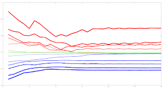
Due to the amount of training data available I decided to look only at a linear model and small neural networks (NN) with a single hidden layer with up to 6 hidden neurons. This choice was motivated by an academic paper I read online about linear models which stated that, as a lower bound, one should have at least 10 training examples for each parameter to be estimated. Other online reading about order flow imbalance (OFI) suggested there is a linear relationship between OFI and price movement. Use of limited size NNs would allow a small amount of non linearity in the relationship. For this investigation I used the Netlab toolbox and Octave. A plot of the learning curves of the classification models tested is shown below. The targets were binary 1/0 for price increases/decreases.

The blue lines show the average training error (y axis) and the red lines show the same average error metric on the held out cross validation data set for each tested model. The thickness of the lines represents the number of neurons in the single hidden layer of the NNs (the thicker the lines, the higher the number of hidden neurons). The horizontal green line shows the error of a generalized linear model (GLM) trained using iteratively reweighted least squares. It can be seen that NN models with 1 and 2 hidden neurons slightly outperform the GLM, with the 2 neuron model having the edge over the 1 neuron model. NN models with 3 or more hidden neurons over fit and underperform the GLM. The NN models were trained using Netlab's functions for Bayesian regularization over the parameters.

Looking at these results it would seem that a 2 neuron NN would be the best choice; however the error differences between the 1 and 2 neuron NNs and GLM are small enough to anticipate that the final classifications (with a basic greater/less than a 0.5 logistic threshold value for long/short) would perhaps be almost identical. 

Investigations into this will be the subject of my next post. 

The code box below gives the working Octave code for the above.

## load data
##training_data = dlmread( 'raw_netlab_training_features' ) ;
##cv_data = dlmread( 'raw_netlab_cv_features' ) ;
training_data = dlmread( 'netlab_training_features_svd' ) ;
cv_data = dlmread( 'netlab_cv_features_svd' ) ;
training_targets = dlmread( 'netlab_training_targets' ) ;
cv_targets = dlmread( 'netlab_cv_targets' ) ;

kk_loop_record = zeros( 30 , 7 ) ;

for kk = 1 : 30
  
## first train a glm model as a base comparison
input_dim = size( training_data , 2 ) ; ## Number of inputs.

net_lin = glm( input_dim , 1 , 'logistic' ) ; ## Create a generalized linear model structure.
options = foptions ; ## Sets default parameters for optimisation routines, for compatibility with MATLAB's foptions()
options(1) = 1 ;  ## change default value
##	OPTIONS(1) is set to 1 to display error values during training. If
##	OPTIONS(1) is set to 0, then only warning messages are displayed.  If
##	OPTIONS(1) is -1, then nothing is displayed.
options(14) = 5 ; ## change default value
##	OPTIONS(14) is the maximum number of iterations for the IRLS
##	algorithm;  default 100.
net_lin = glmtrain( net_lin , options , training_data , training_targets ) ;

## test on cv_data
glm_out = glmfwd( net_lin , cv_data ) ;
## cross-entrophy loss
glm_out_loss = -mean( cv_targets .* log( glm_out )  .+ ( 1 .- cv_targets ) .* log( 1 .- glm_out ) ) ;

kk_loop_record( kk , 7 ) = glm_out_loss ;

## now train an mlp
## Set up vector of options for the optimiser.
nouter = 30 ; ## Number of outer loops.
ninner = 2 ;	## Number of innter loops.
options = foptions ; ## Default options vector.
options( 1 ) = 1 ;	## This provides display of error values.
options( 2 ) = 1.0e-5 ; ## Absolute precision for weights.
options( 3 ) = 1.0e-5 ; ## Precision for objective function.
options( 14 ) = 100 ; ## Number of training cycles in inner loop.

training_learning_curve = zeros( nouter , 6 ) ; 
cv_learning_curve = zeros( nouter , 6 ) ;

for jj = 1 : 6

## Set up network parameters.
nin = size( training_data , 2 ) ; ## Number of inputs.
nhidden = jj ;	## Number of hidden units.
nout = 1 ; ## Number of outputs.
alpha = 0.01 ; ## Initial prior hyperparameter.
aw1 = 0.01 ;
ab1 = 0.01 ;
aw2 = 0.01 ;
ab2 = 0.01 ;

## Create and initialize network weight vector.
prior = mlpprior(nin , nhidden , nout , aw1 , ab1 , aw2 , ab2 ) ;
net = mlp( nin , nhidden , nout , 'logistic' , prior ) ;

## Train using scaled conjugate gradients, re-estimating alpha and beta.
for ii = 1 : nouter
  ## train net
  net = netopt( net , options , training_data , training_targets , 'scg' ) ;
  
  train_out = mlpfwd( net , training_data ) ;
  ## get train error
  ## mse
  ##training_learning_curve( ii ) = mean( ( training_targets .- train_out ).^2 ) ;
  
  ## cross entropy loss
  training_learning_curve( ii , jj ) = -mean( training_targets .* log( train_out )  .+ ( 1 .- training_targets ) .* log( 1 .- train_out ) ) ; 

  cv_out = mlpfwd( net , cv_data ) ;
  ## get cv error
  ## mse
  ##cv_learning_curve( ii ) = mean( ( cv_targets .- cv_out ).^2 ) ;
  
  ## cross entropy loss
  cv_learning_curve( ii , jj ) = -mean( cv_targets .* log( cv_out )  .+ ( 1 .- cv_targets ) .* log( 1 .- cv_out ) ) ; 
  
  ## now update hyperparameters based on evidence
  [ net , gamma ] = evidence( net , training_data , training_targets , ninner ) ;
  
##  fprintf( 1 , '\nRe-estimation cycle ##d:\n' , ii ) ;
##  disp( [ '  alpha = ' , num2str( net.alpha' ) ] ) ;
##  fprintf( 1 , '  gamma =  %8.5f\n\n' , gamma ) ;
##  disp(' ')
##  disp('Press any key to continue.')
  ##pause;
endfor ## ii loop

endfor ## jj loop

kk_loop_record( kk , 1 : 6 ) = cv_learning_curve( end , : ) ;

endfor ## kk loop

plot( training_learning_curve(:,1) , 'b' , 'linewidth' , 1 , cv_learning_curve(:,1) , 'r' , 'linewidth' , 1 , ...
training_learning_curve(:,2) , 'b' , 'linewidth' , 2 , cv_learning_curve(:,2) , 'r' , 'linewidth' , 2 , ...
training_learning_curve(:,3) , 'b' , 'linewidth' , 3 , cv_learning_curve(:,3) , 'r' , 'linewidth' , 3 , ...
training_learning_curve(:,4) , 'b' , 'linewidth' , 4 , cv_learning_curve(:,4) , 'r' , 'linewidth' , 4 , ...
training_learning_curve(:,5) , 'b' , 'linewidth' , 5 , cv_learning_curve(:,5) , 'r' , 'linewidth' , 5 , ...
training_learning_curve(:,6) , 'b' , 'linewidth' , 6 , cv_learning_curve(:,6) , 'r' , 'linewidth' , 6 , ...
ones( size( training_learning_curve , 1 ) , 1 ).*glm_out_loss , 'g' , 'linewidth', 2 ) ;

##  >> mean(kk_loop_record)
##  ans =
##
##     0.6928   0.6927   0.7261   0.7509   0.7821   0.8112   0.6990

##  >> std(kk_loop_record)
##  ans =
##
##     8.5241e-06   7.2869e-06   1.2999e-02   1.5285e-02   2.5769e-02   2.6844e-02   2.2584e-16

A Possible, New Positionbook Indicator?

In my previous post I ended with saying that I would post about some sort of "sentiment indicator" if, and only if, I had something positive to say about my progress on this work. This post is the first on this subject.

The indicator I'm working on is based on the open position ratios data that is available via the Oanda api. For the uninitiated, this data gives the percentage of traders holding long and short positions, and at what price levels, in 14 selected forex pairs and also gold and silver. The data is updated every 20 minutes. I have long felt that there must be some value hidden in this data but the problem is how to extract it.

What I've done is take the percentage values from the (usually) hundreds of separate price levels and sum and normalise them over three defined ranges - levels above/below the high/low of each 20 minute period and the level(s) that span the price range of this period. This is done separately for long and short positions to give a total of 6 percentage figures that sum to 100%. Conceptually, this can be thought of as attaching to the open and close of a 20 minute OHLC bar the 6 percentage position values that were in force at the open and close respectively. The problem is to try and infer the actual, net changes in positions that have taken place over the time period this 20 minute bar was forming. In this way I am trying, if you like, to create a sort of  "skin in the game" indicator as opposed to an indicator derived from order book data, which could be said to be based on traders' current (changeable) intentions as expressed by their open orders and which are subject to shenanigans such as spoofing.

The methodology I've decided on to realise the above is constrained optimization using Octave's fmincon function. The objective function is simply:

    denom = X' * old_pb_net_pos ;
    J = mean( ( new_pb_net_pos .- ( ( X .* old_pb_net_pos ) ./ denom ) ).^2 ) ;

for a multiplicative position value change model where:

• X is a vector of constants that are to be optimised
• old_pb_net_pos is a vector of the 6 percentage values at the open
• new_pb_net_pos is a vector of the 6 percentage values at the close

This is a constrained model because percentage position values at price levels outside the bar range cannot actually increase as a result of trades that take place within the bar range, so the X values for these levels are necessarily constrained to a maximum value of 1 (implying no real, absolute change at these levels). Similarly, all X values must be greater than zero (a zero value would imply a mass exit of all positions at this level, which never actually happens).

The net result of the above is an optimised X vector consisting of multiplicative constants that are multiplied with old_pb_net_pos to achieve new_pb_net_pos according to the logic exemplified in the above objective function. It is these optimised X values from which the underlying, real changes in positions will be inferred and features created. More on this in my next post.

 

Matrix Profile and Weakly Labelled Data - 2nd and Final Update

It has been over three months since my last post, which was intended to be the first in a series of posts on the subject of the title of this post. However, it turned out that the results of my work were underwhelming and so I decided to stop flogging a dead horse and move onto other things. I still have some ideas for using Matrix Profile, but not for the above. These ideas may be the subject of a future blog post.

I subsequently looked at plotting order levels using the data that is available via the Oanda API and I have come up with Octave code to render plots such as this:

where the brighter yellow stripes show ranges where there is an accumulation of sell/buy orders above/below price. These can be interpreted as support/resistance areas. It is normally my practice to post my Octave code, but the code for this plot is quite idiosyncratic and depends very much on the way I have chosen to store the underlying data downloaded from Oanda. As such, I don't think it would be helpful to readers and so I am not posting the code. That said, if there is actually a demand I am more than happy to make it available in a future blog post.

Having done this, it seemed natural to extend it to Open Position Ratios which are also available via the Oanda API. Plotting these levels renders plots that are similar to the plot shown above, but show levels where open long/short positions instead of open orders are accumulated. Although such plots are visually informative, I prefer something more objective, and so for the last few weeks I have been working on using the open position ratios data to construct some sort of sentiment indicator that hopefully could give a heads up to future price movement direction. This is still very much a work in progress which I shall post about if there are noteworthy results.

More in due course.

Matrix Profile and Weakly Labelled Data - Update 1

This is the first post in a short series detailing my recent work following on from my previous post. This post will be about some problems I have had and how I partially solved them.

The main problem was simply the speed at which the code (available from the companion website) seems to run. The first stage Matrix Profile code runs in a few seconds, the second, individual evaluation stage in no more than a few minutes, but the third stage, greedy search, which uses Golden Section Search over the pattern candidates, can take many, many hours. My approach to this was simply to optimise the code to the best of my ability. My optimisations, all in the compute_f_meas.m function, are shown in the following code boxes. This while loop

i = 1;
while true
    
 if i >= length(anno_st)
    break;
 endif
       
first_part = anno_st(1:i);
second_part = anno_st(i+1:end);
bad_st = abs(second_part - anno_st(i)) < sub_len;
second_part = second_part(~bad_st);
anno_st = [first_part; second_part;];
i = i + 1;
      
endwhile

is replaced by this .oct compiled version of the same while loop

#include 
#include 

DEFUN_DLD ( stds_f_meas_while_loop_replace, args, nargout,
"-*- texinfo -*-\n\
@deftypefn {Function File} {} stds_f_meas_while_loop_replace (@var{input_vector,sublen})\n\
This function takes an input vector and a scalar sublen\n\
length. The function sets to zero those elements in the\n\
input vector that are closer to the preceeding value than\n\
sublen. This function replaces a time consuming .m while loop\n\
in the stds compute_f_meas.m function.\n\
@end deftypefn" )

{
octave_value_list retval_list ;
int nargin = args.length () ;

// check the input arguments
if ( nargin != 2 ) // there must be a vector and a scalar sublen
   {
   error ("Invalid arguments. Inputs are a column vector and a scalar value sublen.") ;
   return retval_list ;
   }

if ( args(0).length () < 2 )
   {
   error ("Invalid 1st argument length. Input is a column vector of length > 1.") ;
   return retval_list ;
   }
   
if ( args(1).length () > 1 )
   {
   error ("Invalid 2nd argument length. Input is a scalar value for sublen.") ;
   return retval_list ;
   }
// end of input checking  
  
ColumnVector input = args(0).column_vector_value () ;
double sublen = args(1).double_value () ;
double last_iter ;

// initialise last_iter value
last_iter = input( 0 ) ;
     
for ( octave_idx_type ii ( 1 ) ; ii < args(0).length () ; ii++ )
    {
    
      if ( input( ii ) - last_iter >= sublen )
      {
        last_iter = input( ii ) ;
      }
      else
      {
        input( ii ) = 0.0 ;
      }
      
    } // end for loop
   
retval_list( 0 ) = input ;

return retval_list ;

} // end of function

and called thus

anno_st = stds_f_meas_while_loop_replace( anno_st , sub_len ) ;
anno_st( anno_st == 0 ) = [] ;

This for loop

is_tp = false(length(anno_st), 1);
for i = 1:length(anno_st)
    if anno_ed(i) > length(label)
        anno_ed(i) = length(label);
    end
    if sum(label(anno_st(i):anno_ed(i))) > 0.8*sub_len
        is_tp(i) = true;
    end
end
tp_pre = sum(is_tp);

is replaced by use of cellslices.m and cellfun.m thus

label_length = length( label ) ;
anno_ed( anno_ed > label_length ) = label_length ;
cell_slices = cellslices( label , anno_st , anno_ed ) ;
cell_sums = cellfun( @sum , cell_slices ) ;
tp_pre = sum( cell_sums > 0.8 * sub_len ) ;

and a further for loop

is_tp = false(length(pos_st), 1);
for i = 1:length(pos_st)
    if sum(anno(pos_st(i):pos_ed(i))) > 0.8*sub_len
        is_tp(i) = true;
    end
end
tp_rec = sum(is_tp);

is replaced by

cell_slices = cellslices( anno , pos_st , pos_ed ) ;
cell_sums = cellfun( @sum , cell_slices ) ;
tp_rec = sum( cell_sums > 0.8 * sub_len ) ;

Although the above measurably improves running times, overall the code of the third stage is still sluggish. I have found that the best way to deal with this, on the advice of the original paper's author, is to limit the number of patterns to search for, the "pat_max" variable, to the minimum possible to achieve a satisfactory result. What I mean by this is that if  pat_max = 5 and the result returned also has 5 identified patterns, incrementally increase pat_max until such time that the number of identified patterns is less than pat_max. This does, by necessity, mean running the whole routine a few times, but it is still quicker this way than drastically over estimating pat_max, i.e. choosing a value of say 50 to finally identify maybe only 5/6 patterns.

More in due course.

"Matrix profile: Using Weakly Labeled Time Series to Predict Outcomes" Paper

Back in May of this year I posted about how I had intended to use Matrix Profile (MP) to somehow cluster the "initial balance" of Market Profile charts with a view to getting a heads up on immediately following price action. Since then, my thinking has evolved due to my learning about the paper "Matrix profile: Using Weakly Labeled Time Series to Predict Outcomes" and its companion website. This very much seems to accomplish the same end I had envisaged with my clustering of initial balances, so I am going to try and use this approach instead.

As a preliminary, I have decided to "weakly label" my time series data using the simple code loop shown below.

for ii = 1 : numel( ix )
  
y_values = train_data( ix( ii ) + 1 : ix( ii ) + 19 , 1 ) ;
london_session_ret = y_values( end ) - y_values( 1 ) ;

[ max_y , max_ix ] = max( y_values ) ;
max_long_ex = max_y - y_values( 1 ) ;

[ min_y , min_ix ] = min( y_values ) ;
max_short_ex = min_y - y_values( 1 ) ;

if ( london_session_ret > 0 && ( max_long_ex / ( -1 * max_short_ex ) ) >= 3 && max_ix > min_ix )
 labels( ix( ii ) - 11 : ix( ii ) , 1 ) = 1 ; 
elseif ( london_session_ret < 0 && ( max_short_ex / max_long_ex ) <= -3 && max_ix < min_ix )
  labels( ix( ii ) - 11 : ix( ii ) , 1 ) = -1 ;
endif
 
endfor

What this essentially does (for the long side) is ensure that price is higher at the end of y_values than at the beginning and there is a reward/risk opportunity of at least 3:1 for at least 1 trade during the period covered by the time range of y_values (either the London a.m. session or the combined New York a.m./London p.m. session) following a 7a.m. to 8.50a.m. (local time) formation of an opening Market profile/initial balance and the maximum adverse excursion occurs before the maximum favourable excursion. A typical chart on the long side looks like this.

This would have the "weak" label for a long trade, and the label would be applied to the Market Profile data that immediately precedes this price action. On the other side, a short labelled chart typically looks like this.

As can be seen, trading "against the label" offers few opportunities for profitable entries/exits. My hope is that a "dictionary" of long/short biased Market Profile patterns can be discovered using the ideas/code in the links above. For completeness, the following chart is typical of price action which does not meet the looped code bias for either long or short.

It is easy to envisage trading this type of price action by fading moves that go outside the "value area" of a Market Profile chart.

More in due course.