Monday 9 December 2013

Preliminary Tests of Walk Forward NN Training Idea.

In my suspending work on Brownian bands post I suggested that I wanted to do some preliminary tests of the idea of training a neural net on a walk forward basis. The test I had in mind was a Monte Carlo permutation test as described in David Aronson's book  "Evidence Based Technical Analysis."  Before I go to the trouble of refactoring all my NN code I would like to be sure that, if a NN can be successfully trained in this way, the end result will have been worth the effort. With this aim in mind I used the below implementation of the MC test routine to test the above linked post's idea. The code, as usual, is Octave .oct function C++ code, but taking advantage of Octave's in-built libraries to avoid loops where possible.
DEFUN_DLD ( position_vector_permutation_test, args, nargout, 
"-*- texinfo -*-\n\
@deftypefn {Function File} {} position_vector_permutation_test (@var{returns,position_vector_matrix,iters})\n\
This function takes as inputs a vector of returns, a position vector matrix the columns of which are\n\
the individual position vectors that are to be part of the test and the number of iterations for the test.\n\
If the matrix consists only of one position vector the test performed is the single position vector permuation\n\
test. If there are two or more position vectors the test performed is the data mining bias adjusted permutation\n\
test. The null hypothesis that is tested is that the position vector(s) give results that are no better than those\n\
a random ordering of equivalent net positions would give. The alternative hypothesis is that the position vector(s) give\n\
results that are better than a random ordering would give. The function returns a p-value(s) for the position vector(s)\n\
being tested. If small enough, we can reject the null hypothesis and accept the alternative hypothesis. The returned\n\
p-values are expressed as percentages, i.e 0.05 means a 5% significance value. The test statistic is the sum of returns.\n\
*IMPORTANT NOTE* Apart from basic input argument checks to avoid error messages and seg faults this function does not\n\
check that the returns vector and position vector matrix are properly alligned etc. with regard to accuracy of test results\n\
and makes no assumptions about this. It is the user's responsibility to ensure that the position vector(s) are offset to\n\
match the returns for the particular test in question.\n\
@end deftypefn" )

{
octave_value_list retval_list ; // the return value(s) are p value(s)
int nargin = args.length () ;

// check the input arguments
if ( nargin != 3 )
   {
   error ("Insufficient arguments. Inputs are a returns vector, a position vector matrix and a scalar value for iters.") ;
   return retval_list ;
   }

if ( args(0).length () != args(1).rows () )
   {
   error ("Dimensions mismatch. Length of returns vector should == No.rows of position_vector_matrix.") ;
   return retval_list ;
   }
   
if ( args(2).rows() > 1 )
   {
   error ("Invalid 3rd argument. This should be a scalar value for the number of permutations to perform.") ;
   return retval_list ;
   }
   
if ( args(2).length () != args(2).rows () )
   {
   error ("Invalid 3rd argument. This should be a scalar value for the number of permutations to perform.") ;
   return retval_list ;
   }   

if ( error_state )
   {
   error ("Error state. See usage") ;
   return retval_list ;
   }
// end of input checking

//disable_warning ( "Octave:broadcast" ) ;
set_warning_state ( "Octave:broadcast" , "off" ) ;

RowVector returns = args(0).row_vector_value () ; // Returns vector input
Matrix position_vector = args(1).matrix_value () ; // Positions vector input

// compute the return(s) of the candidate model(s) 
Matrix model_returns ( 1 , position_vector.cols() ) ;
model_returns = returns * position_vector ; // matrix multiplication

// normalised returns multiplier
Matrix normalised_multiplier ( 1 , position_vector.cols() ) ;
normalised_multiplier.fill ( 0.0 ) ;
   
if ( position_vector.cols() > 1 ) // more than one position vector
   {
   for ( octave_idx_type ii (0) ; ii < position_vector.cols() ; ii++ )
       { 
  for ( octave_idx_type jj (0) ; jj < position_vector.rows() ; jj++ )
      {
      normalised_multiplier( 0 , ii ) += fabs( position_vector( jj , ii ) ) ;  
      } // end of jj loop     
  normalised_multiplier( 0 , ii ) = sqrt( position_vector.rows() ) / sqrt( normalised_multiplier( 0 , ii ) ) ; 
       } // end of ii loop   
   } // end of if ( position_vector.cols() > 1 )   
   else // only one position vector
   {
   normalised_multiplier( 0 , 0 ) = 1.0 ;
   }

// use this normalised_multiplier to adjust the model returns
model_returns = product( model_returns , normalised_multiplier ) ;  

// Now do the Monte-Carlo replications
int temp ; 
int k1 ;
int k2 ;
Matrix trial_returns ( 1 , position_vector.cols() ) ;
double max_trial_return ;
Matrix counts ( 1 , position_vector.cols() ) ;
counts.fill ( 0.0 ) ;
MTRand mtrand1 ; // Declare the Mersenne Twister Class - will seed from system time

 for ( octave_idx_type ii (0) ; ii < args(2).int_value() ; ii++ ) // args(2).int_value() is the no. of permutaions to perform 
     {
       trial_returns.fill( 0.0 ) ; // set trial returns to zero

       k1 = args(0).length () - 1 ; // initialise prior to shuffling the returns vector

       while ( k1 > 0 ) // While at least 2 left to shuffle
             {          
             k2 = mtrand1.randInt ( k1 ) ; // Pick an int from 0 through k1 

               if (k2 > k1)     // check if random vector index no. k2 is > than max vector index - should never happen 
                  {
                  k2 = k1 - 1 ; // But this is cheap insurance against disaster if it does happen
                  }

             temp = returns ( k1 ) ;           // allocate the last vector index content to temp
             returns ( k1 ) = returns ( k2 ) ; // allocate random pick to the last vector index
             returns ( k2 ) = temp ;           // allocate temp content to old vector index position of random pick
             k1 = k1 - 1 ;                     // count down 
             }                                 // Shuffling is complete when this while loop exits
             
      // Compute returns for this random shuffle
      trial_returns = returns * position_vector ;
      
      // and now normalise these returns
      trial_returns = product( trial_returns , normalised_multiplier ) ;
      
      max_trial_return = *std::max_element( &trial_returns( 0,0 ), &trial_returns( 0,trial_returns.cols() ) ) ;

        for ( octave_idx_type jj (0) ; jj < trial_returns.cols() ; jj++ )
     {
            if ( max_trial_return >= model_returns(0,jj) ) // If the best random system(s) beats the candidate system(s)
               {
               counts(0,jj) += 1 ; // Count it
               }
     }
     
     } // end of main ii loop

// now write out the results     
Matrix p_values ( 1 , position_vector.cols() ) ;
Matrix iters = args(2).matrix_value () ;   
p_values = quotient( counts , iters ) ; // count divided by number of permutations
 
retval_list(0) = p_values ;
 
set_warning_state ( "Octave:broadcast" , "on" ) ;

return retval_list ; // Return the output to Octave

} // end of function
I am happy to report that the tests were passed with flying colours, although of course this shouldn't really be surprising as there is the benefit of peeking a few days into the future in the historical record.

My next task will be to implement the walk forward version of the NN, which I anticipate will take multiple weeks at a bare minimum to get satisfactorily working Octave code. More in due course.

Friday 6 December 2013

Brownian Oscillator

In my previous post I said I was thinking about an oscillator based on Brownian bands and the lower pane in the video below shows said oscillator in action. The upper pane simply shows the prices with super imposed Brownian bands. The oscillator ranges between 0 and 1 and is effectively a measurement of the randomness of price movement. The calculation is very simple: for consecutive look back periods of 1 to the dominant cycle period a counter is incremented by 1 for each look back length in which price is between the Brownian bands for that look back length, and the sum of this counter is then divided by the dominant cycle period. The logic should be easily discernible from the code given in the code box below. According to this logic the higher the oscillator value the more random price movement is, and the lower the value the higher the "trendiness" of the price series. The value of the oscillator could also be interpreted as the percentage of look back periods which indicate random movement. Nb. I have changed the calculation of the bands to use absolute price differences rather than log differences - I find that this change leads to better behaved bands.

I have not done any testing of this oscillator as an indicator but I think it might have some value as a filter for a trend following system, or as a way of switching between trend following and mean reversion types of systems. The fact that the oscillator values lie in the range 0 to 1 also makes it suitable as an input to a neural net.

The Octave .oct code
DEFUN_DLD ( brownian_oscillator, args, nargout, 
"-*- texinfo -*-\n\
@deftypefn {Function File} {} brownian_oscillator (@var{price,period})\n\
This function takes price and period vector inputs and outputs a value\n\
normalised by the max look back period for the number of look back periods\n\
from 1 to max look back period inclusive for which the price is between\n\
Brownian bands.\n\
@end deftypefn" )

{
octave_value_list retval_list ;
int nargin = args.length () ;

// check the input arguments
if ( nargin != 2 )
   {
   error ( "Invalid arguments. Type help to see usage." ) ;
   return retval_list ;
   }
   
if ( args(0).length () < 50 ) // check length of price vector input
   {
   error ( "Invalid arguments. Type help to see usage." ) ;
   return retval_list ;
   }   
   
if ( args(1).length () != args(0).length () ) // lookback period length argument
   {
   error ( "Invalid arguments. Type help to see usage." ) ;
   return retval_list ;
   }

if ( error_state )
   {
   error ( "Invalid arguments. Type help to see usage." ) ;
   return retval_list ;
   }
// end of input checking   

ColumnVector price = args(0).column_vector_value () ;
ColumnVector period = args(1).column_vector_value () ; 
ColumnVector abs_price_diff = args(0).column_vector_value () ;
ColumnVector osc = args(0).column_vector_value () ; osc(0) = 0.0 ;
double sum ;
double osc_sum ;
double up_bb ;
double low_bb ;
int jj ;

for ( octave_idx_type ii (1) ; ii < 50 ; ii++ ) // initialising loop 
    {
    abs_price_diff(ii) = fabs( price(ii) - price(ii-1) ) ;
    osc(ii) = 0.0 ;
    }
    
for ( octave_idx_type ii (50) ; ii < args(0).length () ; ii++ ) // main loop
    {    
    // initialise calculation values  
    sum = 0.0 ;
    osc_sum = 0.0 ;
    up_bb = 0.0 ;
    low_bb = 0.0 ;

    for ( jj = 1 ; jj < period(ii) + 1 ; jj++ ) // nested jj loop
        {
   
        abs_price_diff(ii) = fabs( price(ii) - price(ii-1) ) ;
        sum += abs_price_diff(ii-jj+1) ;
        up_bb = price(ii-jj) + (sum/double(jj)) * sqrt(double(jj)) ;
        low_bb = price(ii-jj) - (sum/double(jj)) * sqrt(double(jj)) ;
      
        if ( price(ii) <= up_bb && price(ii) >= low_bb )
           {
           osc_sum += 1.0 ;
           }

        } // end of nested jj loop  
    
    osc(ii) = osc_sum / period(ii) ;
    
    } // end of main loop   

    retval_list(0) = osc ;

return retval_list ;

} // end of function

Wednesday 27 November 2013

Brownian Bands revisited?

Further to my most recent post there have been a few anonymous comments suggesting that Brownian bands are more useful than I supposed. In response I have added a contact form to this blog ( on the right ) so these anonymous readers may contact me if they wish. I am curious to learn how they may be using Brownian bands. I might also add that I have thought of creating a new indicator ( a kind of randomness measurement oscillator ) based on the Brownian bands concept.

Sunday 24 November 2013

Suspending Work on Brownian Bands

Recently I have been doing a lot of work looking at various uses of the Brownian bands but I have been unable to come up with anything unique that I feel can help me so for now I am going to discontinue this work. There may be a time in the future when I return to this, but for now the Brownian bands are going to be put on the shelf along with my other indicators.

I have also started to become disillusioned with my attempts at creating a market classifier neural net; I think it may very well be too large a project to complete satisfactorily, so I am going to try something simpler in concept at least. In large part this change of heart is due to some recent reading I have been doing, particularly this article in which I was struck by the phrase

"As an aside, the ideal "trades" formed by the turning points might make a good training set of trades for a neural network-based system. Rather than scanning a chart manually to come up with trades to feed into the neural network, the method described here could be used to automatically find the training set."

Also over on the Mechanical Forex site there is a whole series of articles on neural nets which I have found useful and have given me a new insight. I am now going to ask readers to suspend their disbelief for a few moments while I explain.

Imagine it is a few minutes before the trading open and you have to decide whether to enter long, short or remain out of the market when the market opens. However, unlike any other market participant, the Gods have given you a gift - the ability to see the near future - which means you know the OHLC for today, tomorrow and the next trading day. But, as with all gifts from the Gods, there is a catch - you can only enter and exit trades at the market open; there is no buying the low and selling the high of a candlestick bar or intraday trading permitted by the Gods. What would such a blessed but responsible trader do? How would they make their trade decision? Being responsible s/he might consider the reward to risk ratio and only take a trade if this ratio is greater than one: on the long side the maximum open of tomorrow or the day after minus today's open divided by today's open minus the minimum low of today, tomorrow or the day after: and a similar reasoning for the short side. If neither of these ratios is greater than one, no new trade will be entered today.

The upper pane in the video below shows the coding of such logic. The decision to go long is rendered in blue, short in red and neutral in green. The colour of the bar indicates the action to be taken at the open of the next bar. However, it might be that when a neutral signal is given there is already be a position held, in which case the existing position is held for the duration of the neutral signal. This is effectively an always in the market, stop and reverse signal, and this is shown in the lower pane of the video. To make things slightly easier to see the entry/exit action occurs at the open of a new colour bar, i.e. if the bars change from blue to red the long is exited and the short initiated at the open of the first red bar.
Even with a cursory viewing it can be seen what a great "system" this would be, and using neural nets to create such a "system" is now my ambition.

The plan is simple: roll a moving window along the price series and use the known relationships between bars and indicators within this window to train a locally optimised neural net. The purpose of the training will be to classify the bars as long entry, short entry or neutral as in the chart in the upper pane of the above video. At the hard right edge of the chart the last three bars will be unavailable to the neural net for training purposes, but the hope is that the neural net, sufficiently well trained on all data in the window immediately prior to these three bars, will have predictive ability for them. After all, in the main, market dynamics slowly evolve over a few bars rather than dramatically leap.

Before I embark on this new work there are a few optimisation tests I would like to conduct, and these tests will form the subject matter of my next few posts.

Sunday 17 November 2013

Brownian Bands

For the past few weeks I have been working on the idea presented in my earlier modelling prices using brownian motion post and below is a video of what I have come up with, which I'm calling Brownian Bands. The video shows these bands on the EURUSD forex pair with look back lengths of 1 to 10 bars inclusive, then 15 to 50 in increments of 5, then 50, 100 and 200 and finally 50, 100 and 200 on the whole time series. Each look back length band is the average of all bands from 1 up to and including the look back length band - the details of the implementation can be seen in the code boxes below. The blue band is the upper band, the red is the lower and the green is the mid point of the two.

           
Non-embedded view.

This following chart shows an adaptive look back length implementation, the look back length being determined by a period vector input to the function, which in this case is the dominant cycle period.
These adaptive Brownian bands can be compared with the equivalent adaptive Bollinger bands shown in this next chart.
For my intended purpose of separating out returns into distribution bins the Brownian bands seem to be superior. There are 3 distinct bins: above the upper band, below the lower band and between the bands, whereas with the Bollinger bands the vast majority of returns would be lumped into just one bin - between the bands. Of course the Brownian bands could be used to create a system indicator just as Bollinger bands can be, and if any readers test this idea I would be intrigued to hear of your results. However, should you choose to do this there is a major caveat you should be aware of. The calculation of the Brownian bands is based on the natural log of actual price, which means you should be very wary of test results on any back adjusted price series such as futures and adjusted stock prices. In fact I would go as far to say that the code given below should not be used as is on such price series. It is for this reason that I have been using forex price series in my own tests so far, but I will surely get around to adjusting the given code in due course.

Now for the code. This first code box shows a hard-coded, unrolled loop version for look back lengths up to and including 25 for the benefit of a reader who requested a clearer exposition of the method than was given in my earlier post, which was vectorised Octave code. All the code below is C++ as used in Octave .oct files.
DEFUN_DLD ( brownian_bands_25, args, nargout, 
"-*- texinfo -*-\n\
@deftypefn {Function File} {} brownian_bands_25 (@var{price,period})\n\
This function takes a price vector input and a value for the tick\n\
size of the instrument and outputs upper and lower bands based on\n\
the concept of Brownian motion. The bands are the average of look\n\
back periods of 1 to 25 bars inclusive of the relevant calculations.\n\
@end deftypefn" )

{
octave_value_list retval_list ;
int nargin = args.length () ;

// check the input arguments
if ( nargin != 2 )
   {
   error ( "Invalid arguments. Type help to see usage." ) ;
   return retval_list ;
   }

if ( args(0).length () < 21 )
   {
   error ( "Invalid arguments. Type help to see usage." ) ;
   return retval_list ;
   }
   
if ( args(1).length () != 1 )
   {
   error ( "Invalid arguments. Type help to see usage." ) ;
   return retval_list ;
   }   

if ( error_state )
   {
   error ( "Invalid arguments. Type help to see usage." ) ;
   return retval_list ;
   }
// end of input checking   

ColumnVector price = args(0).column_vector_value () ;
double tick_size = args(1).double_value() ;
ColumnVector abs_log_price_diff = args(0).column_vector_value () ;
ColumnVector upper_band = args(0).column_vector_value () ;
ColumnVector lower_band = args(0).column_vector_value () ;
ColumnVector mid_band = args(0).column_vector_value () ;
double sum ;

double up_1 ;
double low_1 ;

double up_2 ;
double low_2 ;
double sqrt_2 = sqrt(2.0) ; // pre-calculated for speed optimisation

double up_3 ;
double low_3 ;
double sqrt_3 = sqrt(3.0) ; // pre-calculated for speed optimisation

double up_4 ;
double low_4 ;
double sqrt_4 = sqrt(4.0) ; // pre-calculated for speed optimisation

double up_5 ;
double low_5 ;
double sqrt_5 = sqrt(5.0) ; // pre-calculated for speed optimisation

double up_6 ;
double low_6 ;
double sqrt_6 = sqrt(6.0) ; // pre-calculated for speed optimisation

double up_7 ;
double low_7 ;
double sqrt_7 = sqrt(7.0) ; // pre-calculated for speed optimisation

double up_8 ;
double low_8 ;
double sqrt_8 = sqrt(8.0) ; // pre-calculated for speed optimisation

double up_9 ;
double low_9 ;
double sqrt_9 = sqrt(9.0) ; // pre-calculated for speed optimisation

double up_10 ;
double low_10 ;
double sqrt_10 = sqrt(10.0) ; // pre-calculated for speed optimisation

double up_11 ;
double low_11 ;
double sqrt_11 = sqrt(11.0) ; // pre-calculated for speed optimisation

double up_12 ;
double low_12 ;
double sqrt_12 = sqrt(12.0) ; // pre-calculated for speed optimisation

double up_13 ;
double low_13 ;
double sqrt_13 = sqrt(13.0) ; // pre-calculated for speed optimisation

double up_14 ;
double low_14 ;
double sqrt_14 = sqrt(14.0) ; // pre-calculated for speed optimisation

double up_15 ;
double low_15 ;
double sqrt_15 = sqrt(15.0) ; // pre-calculated for speed optimisation

double up_16 ;
double low_16 ;
double sqrt_16 = sqrt(16.0) ; // pre-calculated for speed optimisation

double up_17 ;
double low_17 ;
double sqrt_17 = sqrt(17.0) ; // pre-calculated for speed optimisation

double up_18 ;
double low_18 ;
double sqrt_18 = sqrt(18.0) ; // pre-calculated for speed optimisation

double up_19 ;
double low_19 ;
double sqrt_19 = sqrt(19.0) ; // pre-calculated for speed optimisation

double up_20 ;
double low_20 ;
double sqrt_20 = sqrt(20.0) ; // pre-calculated for speed optimisation

double up_21 ;
double low_21 ;
double sqrt_21 = sqrt(21.0) ; // pre-calculated for speed optimisation

double up_22 ;
double low_22 ;
double sqrt_22 = sqrt(22.0) ; // pre-calculated for speed optimisation

double up_23 ;
double low_23 ;
double sqrt_23 = sqrt(23.0) ; // pre-calculated for speed optimisation

double up_24 ;
double low_24 ;
double sqrt_24 = sqrt(24.0) ; // pre-calculated for speed optimisation

double up_25 ;
double low_25 ;
double sqrt_25 = sqrt(25.0) ; // pre-calculated for speed optimisation

for ( octave_idx_type ii (1) ; ii < 25 ; ii++ ) // initialising loop 
    {
    abs_log_price_diff(ii) = fabs( log( price(ii) ) - log( price(ii-1) ) ) ;
    }
    
for ( octave_idx_type ii (25) ; ii < args(0).length () ; ii++ ) // main loop
    {
      
    abs_log_price_diff(ii) = fabs( log( price(ii) ) - log( price(ii-1) ) ) ;

    sum = abs_log_price_diff(ii) ;
    up_1 = exp( log( price(ii-1) ) + sum ) ;
    low_1 = exp( log( price(ii-1) ) - sum ) ;

    sum += abs_log_price_diff(ii-1) ;
    up_2 = exp( log( price(ii-2) ) + (sum/2.0) * sqrt_2 ) ;
    low_2 = exp( log( price(ii-2) ) - (sum/2.0) * sqrt_2 ) ;

    sum += abs_log_price_diff(ii-2) ;
    up_3 = exp( log( price(ii-3) ) + (sum/3.0) * sqrt_3 ) ;
    low_3 = exp( log( price(ii-3) ) - (sum/3.0) * sqrt_3 ) ;
    
    sum += abs_log_price_diff(ii-3) ;
    up_4 = exp( log( price(ii-4) ) + (sum/4.0) * sqrt_4 ) ;
    low_4 = exp( log( price(ii-4) ) - (sum/4.0) * sqrt_4 ) ;

    sum += abs_log_price_diff(ii-4) ;
    up_5 = exp( log( price(ii-5) ) + (sum/5.0) * sqrt_5 ) ;
    low_5 = exp( log( price(ii-5) ) - (sum/5.0) * sqrt_5 ) ;    

    sum += abs_log_price_diff(ii-5) ;
    up_6 = exp( log( price(ii-6) ) + (sum/6.0) * sqrt_6 ) ;
    low_6 = exp( log( price(ii-6) ) - (sum/6.0) * sqrt_6 ) ;
    
    sum += abs_log_price_diff(ii-6) ;
    up_7 = exp( log( price(ii-7) ) + (sum/7.0) * sqrt_7 ) ;
    low_7 = exp( log( price(ii-7) ) - (sum/7.0) * sqrt_7 ) ;
    
    sum += abs_log_price_diff(ii-7) ;
    up_8 = exp( log( price(ii-8) ) + (sum/8.0) * sqrt_8 ) ;
    low_8 = exp( log( price(ii-8) ) - (sum/8.0) * sqrt_8 ) ;
    
    sum += abs_log_price_diff(ii-8) ;
    up_9 = exp( log( price(ii-9) ) + (sum/9.0) * sqrt_9 ) ;
    low_9 = exp( log( price(ii-9) ) - (sum/9.0) * sqrt_9 ) ;
    
    sum += abs_log_price_diff(ii-9) ;
    up_10 = exp( log( price(ii-10) ) + (sum/10.0) * sqrt_10 ) ;
    low_10 = exp( log( price(ii-10) ) - (sum/10.0) * sqrt_10 ) ;
    
    sum += abs_log_price_diff(ii-10) ;
    up_11 = exp( log( price(ii-11) ) + (sum/11.0) * sqrt_11 ) ;
    low_11 = exp( log( price(ii-11) ) - (sum/11.0) * sqrt_11 ) ;
    
    sum += abs_log_price_diff(ii-11) ;
    up_12 = exp( log( price(ii-12) ) + (sum/12.0) * sqrt_12 ) ;
    low_12 = exp( log( price(ii-12) ) - (sum/12.0) * sqrt_12 ) ;
    
    sum += abs_log_price_diff(ii-12) ;
    up_13 = exp( log( price(ii-13) ) + (sum/13.0) * sqrt_13 ) ;
    low_13 = exp( log( price(ii-13) ) - (sum/13.0) * sqrt_13 ) ;
    
    sum += abs_log_price_diff(ii-13) ;
    up_14 = exp( log( price(ii-14) ) + (sum/14.0) * sqrt_14 ) ;
    low_14 = exp( log( price(ii-14) ) - (sum/14.0) * sqrt_14 ) ;
    
    sum += abs_log_price_diff(ii-14) ;
    up_15 = exp( log( price(ii-15) ) + (sum/15.0) * sqrt_15 ) ;
    low_15 = exp( log( price(ii-15) ) - (sum/15.0) * sqrt_15 ) ;
    
    sum += abs_log_price_diff(ii-15) ;
    up_16 = exp( log( price(ii-16) ) + (sum/16.0) * sqrt_16 ) ;
    low_16 = exp( log( price(ii-16) ) - (sum/16.0) * sqrt_16 ) ;
    
    sum += abs_log_price_diff(ii-16) ;
    up_17 = exp( log( price(ii-17) ) + (sum/17.0) * sqrt_17 ) ;
    low_17 = exp( log( price(ii-17) ) - (sum/17.0) * sqrt_17 ) ;
    
    sum += abs_log_price_diff(ii-17) ;
    up_18 = exp( log( price(ii-18) ) + (sum/18.0) * sqrt_18 ) ;
    low_18 = exp( log( price(ii-18) ) - (sum/18.0) * sqrt_18 ) ;
    
    sum += abs_log_price_diff(ii-18) ;
    up_19 = exp( log( price(ii-19) ) + (sum/19.0) * sqrt_19 ) ;
    low_19 = exp( log( price(ii-19) ) - (sum/19.0) * sqrt_19 ) ;
    
    sum += abs_log_price_diff(ii-19) ;
    up_20 = exp( log( price(ii-20) ) + (sum/20.0) * sqrt_20 ) ;
    low_20 = exp( log( price(ii-20) ) - (sum/20.0) * sqrt_20 ) ;
    
    sum += abs_log_price_diff(ii-20) ;
    up_21 = exp( log( price(ii-21) ) + (sum/21.0) * sqrt_21 ) ;
    low_21 = exp( log( price(ii-21) ) - (sum/21.0) * sqrt_21 ) ;
    
    sum += abs_log_price_diff(ii-21) ;
    up_22 = exp( log( price(ii-22) ) + (sum/22.0) * sqrt_22 ) ;
    low_22 = exp( log( price(ii-22) ) - (sum/22.0) * sqrt_22 ) ;
    
    sum += abs_log_price_diff(ii-22) ;
    up_23 = exp( log( price(ii-23) ) + (sum/23.0) * sqrt_23 ) ;
    low_23 = exp( log( price(ii-23) ) - (sum/23.0) * sqrt_23 ) ;
    
    sum += abs_log_price_diff(ii-23) ;
    up_24 = exp( log( price(ii-24) ) + (sum/24.0) * sqrt_24 ) ;
    low_24 = exp( log( price(ii-24) ) - (sum/24.0) * sqrt_24 ) ;
    
    sum += abs_log_price_diff(ii-24) ;
    up_25 = exp( log( price(ii-25) ) + (sum/25.0) * sqrt_25 ) ;
    low_25 = exp( log( price(ii-25) ) - (sum/25.0) * sqrt_25 ) ;
    
    upper_band(ii) = (up_1+up_2+up_3+up_4+up_5+up_6+up_7+up_8+up_9+up_10+up_11+up_12+up_13+up_14+up_15+up_16+up_17+up_18+up_19+up_20+up_21+up_22+up_23+up_24+up_25)/25.0 ;
    lower_band(ii) = (low_1+low_2+low_3+low_4+low_5+low_6+low_7+low_8+low_9+low_10+low_11+low_12+low_13+low_14+low_15+low_16+low_17+low_18+low_19+low_20+low_21+low_22+low_23+up_24+low_25)/25.0 ;
    
    // round the upper_band up to the nearest tick
    upper_band(ii) = ceil( upper_band(ii)/tick_size ) * tick_size ;
    
    // round the lower_band down to the nearest tick
    lower_band(ii) = floor( lower_band(ii)/tick_size ) * tick_size ;
    
    mid_band(ii) = ( upper_band(ii) + lower_band(ii) ) / 2.0 ;
    
    } // end of main loop   

    retval_list(2) = mid_band ;
    retval_list(1) = lower_band ;
    retval_list(0) = upper_band ;

return retval_list ;

} // end of function
This next code box contains code for an adjustable look back length, the length being a user input to the function. This code wraps the above unrolled loop into a nested loop.
DEFUN_DLD ( brownian_bands_adjustable, args, nargout, 
"-*- texinfo -*-\n\
@deftypefn {Function File} {} brownian_bands_adjustable (@var{price,lookback,tick_size})\n\
This function takes a price vector input, a value for the lookback\n\
length and a value for the tick size of the instrument and outputs\n\
upper and lower bands based on the concept of Brownian motion. The bands\n\
are the average of lookback period bands from 1 to lookback length.\n\
@end deftypefn" )

{
octave_value_list retval_list ;
int nargin = args.length () ;

// check the input arguments
if ( nargin != 3 )
   {
   error ( "Invalid arguments. Type help to see usage." ) ;
   return retval_list ;
   }
   
if ( args(1).length () != 1 ) // lookback length argument
   {
   error ( "Invalid arguments. Type help to see usage." ) ;
   return retval_list ;
   }
   
double lookback = args(1).double_value() ;   

if ( args(0).length () < lookback ) // check length of price vector input
   {
   error ( "Invalid arguments. Type help to see usage." ) ;
   return retval_list ;
   }
   
if ( args(2).length () != 1 ) // tick size
   {
   error ( "Invalid arguments. Type help to see usage." ) ;
   return retval_list ;
   }   
   
if ( error_state )
   {
   error ( "Invalid arguments. Type help to see usage." ) ;
   return retval_list ;
   }
// end of input checking   

ColumnVector price = args(0).column_vector_value () ;
double tick_size = args(2).double_value() ;
ColumnVector abs_log_price_diff = args(0).column_vector_value () ;
ColumnVector upper_band = args(0).column_vector_value () ;
ColumnVector lower_band = args(0).column_vector_value () ;
ColumnVector mid_band = args(0).column_vector_value () ;
double sum ;
double up_bb ;
double low_bb ;
int jj ;

for ( octave_idx_type ii (1) ; ii < lookback ; ii++ ) // initialising loop 
    {
    abs_log_price_diff(ii) = fabs( log( price(ii) ) - log( price(ii-1) ) ) ;
    }
    
for ( octave_idx_type ii (lookback) ; ii < args(0).length () ; ii++ ) // main loop
    {    
    // initialise calculation values  
    sum = 0.0 ;
    up_bb = 0.0 ;
    low_bb = 0.0 ;

    for ( jj = 1 ; jj < lookback + 1 ; jj++ ) // nested jj loop
        {
   
 abs_log_price_diff(ii) = fabs( log( price(ii) ) - log( price(ii-1) ) ) ;
        sum += abs_log_price_diff(ii-jj+1) ;
        up_bb += exp( log( price(ii-jj) ) + (sum/double(jj)) * sqrt(double(jj)) ) ;
        low_bb += exp( log( price(ii-jj) ) - (sum/double(jj)) * sqrt(double(jj)) ) ;  

 } // end of nested jj loop  
    
    upper_band(ii) = up_bb / lookback ;
    lower_band(ii) = low_bb / lookback ;
    
    // round the upper_band up to the nearest tick
    upper_band(ii) = ceil( upper_band(ii)/tick_size ) * tick_size ;
    
    // round the lower_band down to the nearest tick
    lower_band(ii) = floor( lower_band(ii)/tick_size ) * tick_size ;
    
    mid_band(ii) = ( upper_band(ii) + lower_band(ii) ) / 2.0 ;
    
    } // end of main loop   

    retval_list(2) = mid_band ;
    retval_list(1) = lower_band ;
    retval_list(0) = upper_band ;

return retval_list ;

} // end of function
Finally, this code is the adaptive look back version where the length of the look back is contained in a vector which is also a user input.
DEFUN_DLD ( brownian_bands_adaptive, args, nargout, 
"-*- texinfo -*-\n\
@deftypefn {Function File} {} brownian_bands_adaptive (@var{price,period,tick_size})\n\
This function takes price and period vector inputs & a value for the tick\n\
size of the instrument and outputs upper and lower bands based on\n\
the concept of Brownian motion. The bands are adaptive averages of look\n\
back lengths of 1 to period bars inclusive.\n\
@end deftypefn" )

{
octave_value_list retval_list ;
int nargin = args.length () ;

// check the input arguments
if ( nargin != 3 )
   {
   error ( "Invalid arguments. Type help to see usage." ) ;
   return retval_list ;
   }
   
if ( args(0).length () < 50 ) // check length of price vector input
   {
   error ( "Invalid arguments. Type help to see usage." ) ;
   return retval_list ;
   }   
   
if ( args(1).length () != args(0).length () ) // lookback period length argument
   {
   error ( "Invalid arguments. Type help to see usage." ) ;
   return retval_list ;
   }
      
if ( args(2).length () != 1 ) // tick size
   {
   error ( "Invalid arguments. Type help to see usage." ) ;
   return retval_list ;
   }   
   
if ( error_state )
   {
   error ( "Invalid arguments. Type help to see usage." ) ;
   return retval_list ;
   }
// end of input checking   

ColumnVector price = args(0).column_vector_value () ;
ColumnVector period = args(1).column_vector_value () ; 
double tick_size = args(2).double_value() ;
ColumnVector abs_log_price_diff = args(0).column_vector_value () ;
ColumnVector upper_band = args(0).column_vector_value () ;
ColumnVector lower_band = args(0).column_vector_value () ;
ColumnVector mid_band = args(0).column_vector_value () ;
double sum ;
double up_bb ;
double low_bb ;
int jj ;

for ( octave_idx_type ii (1) ; ii < 50 ; ii++ ) // initialising loop 
    {
    abs_log_price_diff(ii) = fabs( log( price(ii) ) - log( price(ii-1) ) ) ;
    }
    
for ( octave_idx_type ii (50) ; ii < args(0).length () ; ii++ ) // main loop
    {    
    // initialise calculation values  
    sum = 0.0 ;
    up_bb = 0.0 ;
    low_bb = 0.0 ;

    for ( jj = 1 ; jj < period(ii) + 1 ; jj++ ) // nested jj loop
        {
   
 abs_log_price_diff(ii) = fabs( log( price(ii) ) - log( price(ii-1) ) ) ;
        sum += abs_log_price_diff(ii-jj+1) ;
        up_bb += exp( log( price(ii-jj) ) + (sum/double(jj)) * sqrt(double(jj)) ) ;
        low_bb += exp( log( price(ii-jj) ) - (sum/double(jj)) * sqrt(double(jj)) ) ;  

 } // end of nested jj loop  
    
    upper_band(ii) = up_bb / period(ii) ;
    lower_band(ii) = low_bb / period(ii) ;
    
    // round the upper_band up to the nearest tick
    upper_band(ii) = ceil( upper_band(ii)/tick_size ) * tick_size ;
    
    // round the lower_band down to the nearest tick
    lower_band(ii) = floor( lower_band(ii)/tick_size ) * tick_size ;
    
    mid_band(ii) = ( upper_band(ii) + lower_band(ii) ) / 2.0 ;
    
    } // end of main loop   

    retval_list(2) = mid_band ;
    retval_list(1) = lower_band ;
    retval_list(0) = upper_band ;

return retval_list ;

} // end of function
Due to formatting issues on Blogger none of the code boxes contain the required header statements, which should be:-

#include octave/oct.h
#include octave/dColVector.h
#include math.h

with the customary < before "octave" and "math" and > after ".h"

Thursday 31 October 2013

Exploratory Data Analysis of Brownian Motion Model

For my first steps in investigating the earlier proposed Brownian motion model I thought I would use some Exploratory Data Analysis techniques. I have initially decided to use look back periods of 5 bars and 21 bars; the 5 bar on daily data being a crude attempt to capture the essence of weekly price movement and the 21 bar to capture the majority of dominant cycle periods in daily data, with both parameters also being non optimised Fibonacci numbers. Using the two channels over price bars that these create it is possible to postulate nine separate and distinct price "regimes" using combinations of the criteria of being above, within or below each channel.

The use of these "regimes" is to bin normalised price change at time t into nine separate distributions, the normalising factor being the 5 bar simple moving average of absolute natural log differences at time t-1 and the choice of regime being determined by the position of the close at t-1. The rationale behind basing these metrics on preceding bars is explained in this earlier post and the implementation made clear in the code box at the end of this post. The following 4 charts are Box plots of these nine distributions, in consecutive order, for the EURUSD, GBPUSD, USDCHF and USDYEN  forex pairs:


Looking at these, I'm struck by two things. Firstly, the middle three box plots are for regimes where price is in the 21 bar channel, and numbering from the left, boxes 4, 5 and 6 are below the 5 bar channel, in it and above it. These are essentially different degrees of a sideways market and it can be seen that there are far more outliers here than in the other box plots, perhaps indicating the tendency for high volatility breakouts to occur more frequently in sideways markets.

The second thing that is striking is, again numbering from the left, box plots 3 and 7. These are regimes below the 21 bar and above the 5 bar; and above the 21 bar and below the 5 bar - essentially the distributions for reactions against prevailing trends on the 21 bar time scale. Here it can be seen that there are far fewer outliers and generally shorter whiskers, indicating the tendency for reactions against trends to be less volatile in nature.

It is encouraging to see that there are such differences in these box plots as it suggests that my idea of binning does separate out the different price change characteristics. However, I believe things can be improved a bit in this regard and this will form the subject matter of my next post.
clear all

data = load("-ascii","usdyen") ;
close = data(:,7) ;
logdiff = [ 0 ; diff( log(close) ) ] ;
abslogdiff = abs( logdiff ) ;

sq_rt = sqrt( 5 ) ;
sma5 = sma(abslogdiff,5) ;
ub5 = exp(shift(log(close),5).+(sma5.*sq_rt)) ;
lb5 = exp(shift(log(close),5).-(sma5.*sq_rt)) ;

sq_rt = sqrt( 21 ) ;
sma21 = sma(abslogdiff,21) ;
ub21 = exp(shift(log(close),21).+(sma21.*sq_rt)) ;
lb21 = exp(shift(log(close),21).-(sma21.*sq_rt)) ;

% allocate close bar to a market_type
market_type = zeros( size(close,1) , 1 ) ;

% above ub21 **********************
val_1 = close > ub21 ;
val_2 = close > ub5 ;
matches = val_1 .* val_2 ;
ix = find( matches == 1 ) ;
market_type( ix , 1 ) = 4 ;

val_1 = close > ub21 ;
val_2 = close <= ub5 ;
val_3 = close >= lb5 ;
matches = val_1 .* val_2 .* val_3 ;
ix = find( matches == 1 ) ;
market_type( ix , 1 ) = 3 ;

val_1 = close > ub21 ;
val_2 = close < lb5 ;
matches = val_1 .* val_2 ;
ix = find( matches == 1 ) ;
market_type( ix , 1 ) = 2 ;
%**********************************

% below lb21 **********************
val_1 = close < lb21 ;
val_2 = close < lb5 ;
matches = val_1 .* val_2 ;
ix = find( matches == 1 ) ;
market_type( ix , 1 ) = -4 ;

val_1 = close < lb21 ;
val_2 = close <= ub5 ;
val_3 = close >= lb5 ;
matches = val_1 .* val_2 .* val_3 ;
ix = find( matches == 1 ) ;
market_type( ix , 1 ) = -3 ;

val_1 = close < lb21 ;
val_2 = close > ub5 ;
matches = val_1 .* val_2 ;
ix = find( matches == 1 ) ;
market_type( ix , 1 ) = -2 ;
%**********************************

% between ub21 & lb21**************
val_1 = close <= ub21 ;
val_2 = close >= lb21 ;
val_3 = close > ub5 ;
matches = val_1 .* val_2 .* val_3 ;
ix = find( matches == 1 ) ;
market_type( ix , 1 ) = 1 ;

val_1 = close <= ub21 ;
val_2 = close >= lb21 ;
val_3 = close < lb5 ;
matches = val_1 .* val_2 .* val_3 ;
ix = find( matches == 1 ) ;
market_type( ix , 1 ) = -1 ;
%**********************************

% now allocate to bins
normalised_logdiffs = logdiff ./ shift( sma5 , 1 ) ;

% shift market_type to agree with normalised_logdiffs
shifted_market_type = shift( market_type , 1 ) ;

bin_4 = normalised_logdiffs( find( shifted_market_type(30:end,1) == 4 ) , 1 ) ;
bin_3 = normalised_logdiffs( find( shifted_market_type(30:end,1) == 3 ) , 1 ) ;
bin_2 = normalised_logdiffs( find( shifted_market_type(30:end,1) == 2 ) , 1 ) ;
bin_1 = normalised_logdiffs( find( shifted_market_type(30:end,1) == 1 ) , 1 ) ;
bin_0 = normalised_logdiffs( find( shifted_market_type(30:end,1) == 0 ) , 1 ) ;
bin_1m = normalised_logdiffs( find( shifted_market_type(30:end,1) == -1 ) , 1 ) ;
bin_2m = normalised_logdiffs( find( shifted_market_type(30:end,1) == -2 ) , 1 ) ;
bin_3m = normalised_logdiffs( find( shifted_market_type(30:end,1) == -3 ) , 1 ) ;
bin_4m = normalised_logdiffs( find( shifted_market_type(30:end,1) == -4 ) , 1 ) ;

y_axis_max = max( normalised_logdiffs(30:end,1) ) ;
y_axis_min = min( normalised_logdiffs(30:end,1) ) ;

clf ;
subplot(191) ; boxplot(bin_4m,NOTCHED=1) ; ylim([y_axis_min y_axis_max]) ;
subplot(192) ; boxplot(bin_3m,NOTCHED=1) ; ylim([y_axis_min y_axis_max]) ;
subplot(193) ; boxplot(bin_2m,NOTCHED=1) ; ylim([y_axis_min y_axis_max]) ;
subplot(194) ; boxplot(bin_1m,NOTCHED=1) ; ylim([y_axis_min y_axis_max]) ;
subplot(195) ; boxplot(bin_0,NOTCHED=1) ; ylim([y_axis_min y_axis_max]) ;
subplot(196) ; boxplot(bin_1,NOTCHED=1) ; ylim([y_axis_min y_axis_max]) ;
subplot(197) ; boxplot(bin_2,NOTCHED=1) ; ylim([y_axis_min y_axis_max]) ;
subplot(198) ; boxplot(bin_3,NOTCHED=1) ; ylim([y_axis_min y_axis_max]) ;
subplot(199) ; boxplot(bin_4,NOTCHED=1) ; ylim([y_axis_min y_axis_max]) ;

Sunday 27 October 2013

Modelling Prices Using Brownian Motion.

As stated in my previous post I'm going to rewrite my data generation code for future use in online training of neural nets, and the approach I'm going to take is to combine the concept of Brownian motion and the ideas contained in my earlier Creation of Synthetic Data post.

The basic premise, taken from Brownian motion, is that the natural log of price changes, on average, at a rate proportional to the square root of time. Take, for example, a period of 5 leading up to the "current bar." If we take a 5 period simple moving average of the absolute differences of the log of prices over this period, we get a value for the average 1 bar price movement over this period. This value is then multiplied by the square root of 5 and added to and subtracted from the price 5 days ago to get an upper and lower bound for the current bar. If the current bar lies between the bounds, we say that price movement over the last 5 periods is consistent with Brownian motion and declare an absence of trend, i.e. a sideways market. If the current bar lies outside the bounds, we declare that price movement over the last 5 bars is not consistent with Brownian motion and that a trend is in force, either up or down depending on which bound the current bar is beyond. The following 3 charts show this concept in action, for consecutive periods of 5, 13 and 21, taken from the Fibonacci Sequence:


where yellow is the closing price, blue is the upper bound and red the lower bound. It is easy to imagine many uses for this in terms of indicator creation, but I intend to use the bounds to assign a score of price randomness/trendiness over various combined periods to assign price movement to bins for subsequent Monte Carlo creation of synthetic price series. Interested readers are invited to read the above linked Creation of Synthetic Data post for a review of this methodology.

The rough working Octave code that produced the above charts is given below.
clear all

data = load("-ascii","eurusd") ;
% length = input( 'Enter length of look back for calculations: ' ) ;
% sq_rt = sqrt( length ) ;
close = data(:,7) ;
abslogdiff = abs( [ 0 ; diff( log(close) ) ] ) ;

lngth = 3 ;
sq_rt = sqrt( lngth ) ;
sma3 = sma(abslogdiff,lngth) ;
ub = exp(shift(log(close),lngth).+(sma3.*sq_rt)) ;
lb = exp(shift(log(close),lngth).-(sma3.*sq_rt)) ;

all_ub = ub ;
all_lb = lb ;

lngth = 5 ;
sq_rt = sqrt( lngth ) ;
sma5 = sma(abslogdiff,5) ;
ub = exp(shift(log(close),lngth).+(sma5.*sq_rt)) ;
lb = exp(shift(log(close),lngth).-(sma5.*sq_rt)) ;

all_ub = all_ub .+ ub ;
all_lb = all_lb .+ lb ;

lngth = 8 ;
sq_rt = sqrt( lngth ) ;
sma8 = sma(abslogdiff,lngth) ;
ub = exp(shift(log(close),lngth).+(sma8.*sq_rt)) ;
lb = exp(shift(log(close),lngth).-(sma8.*sq_rt)) ;

all_ub = all_ub .+ ub ;
all_lb = all_lb .+ lb ;

lngth = 13 ;
sq_rt = sqrt( lngth ) ;
sma13 = sma(abslogdiff,lngth) ;
ub = exp(shift(log(close),lngth).+(sma13.*sq_rt)) ;
lb = exp(shift(log(close),lngth).-(sma13.*sq_rt)) ;

all_ub = all_ub .+ ub ;
all_lb = all_lb .+ lb ;

lngth = 21 ;
sq_rt = sqrt( lngth ) ;
sma21 = sma(abslogdiff,lngth) ;
ub = exp(shift(log(close),lngth).+(sma21.*sq_rt)) ;
lb = exp(shift(log(close),lngth).-(sma21.*sq_rt)) ;

all_ub = ( all_ub .+ ub ) ./ 5 ;
all_lb = ( all_lb .+ lb ) ./ 5 ;

 plot(close(1850:2100,1),'y',ub(1850:2100,1),'c',lb(1850:2100,1),'r')
%plot(close,'y',ub,'c',lb,'r')

Saturday 26 October 2013

Change of Direction in Neural Net Training.

Up till now when training my neural net classifier I have been using what I call my "idealised" data, which is essentially a model for prices comprised of a sine wave along with a linear trend. In my recent work on Savitzky-Golay filters I wanted to increase the amount of available training data but have run into a problem - the size of my data files has become so large that I'm exhausting the memory available to me in my Octave software install. To overcome this problem I have decided to convert my NN training to an online regime rather than loading csv data files for mini-batch gradient descent training - in fact what I envisage doing would perhaps be best described as online mini-batch training.

To do this will require a fairly major rewrite of my data generation code and I think I will take the opportunity to make this data generation more realistic than the sine wave and trend model I am currently using. Apart from the above mentioned memory problem, this decision has been prompted by an e-mail exchange I have recently had with a reader of this blog and some online reading I have recently been doing, such as mixed regime simulation, training a simple neural network to recognise different regimes in financial time series, neural networks in trading, random subspace optimisation and profitable hidden and markovian coupling. At the moment it is my intention to revisit my earlier posts here and here and use/extend the ideas contained therein. This means that for the nearest future my work on Savitzky-Golay filters is temporarily halted.

Tuesday 15 October 2013

Code refactoring didn't work.

In my previous post I said that I was going to refactor code to use my existing, trained classification neural net with Savitzky-Golay filter inputs in the hope that this might show some improvement. I have to report that this was an abysmal failure and I suppose it was a bit naive to have ever expected that it would work. It looks like I will have to explicitly train a new neural network to take advantage of Savitzky-Golay filter features.

Sunday 6 October 2013

Update on Savitzky-Golay Filters

For the past couple of weeks I have been playing around with Savitzky-Golay filters with a hope of creating a moving endpoint regression line as a form of zero lag smoothing, but unfortunately I have been unable to come up with anything that is remotely satisfying and I think I'm going to abandon this for now. My view at the moment is that SG filters' utility, for my purposes at least, is limited to feature extraction via the polynomial coefficients to get the 2nd, 3rd and 4th derivatives as inputs for my Neural net classifier.

To do this will require a time consuming retraining period, so before I embark on this I'm going to use what I think will be an immediately useful SG filter application. In a previous post readers can see three screenshots of moving windows of my idealised price series with SG filters overlaid. The SG filters follow these windowed "prices" so closely that I think SG filters more or less == windowed idealised prices and features derived there from. However, when it comes to applying my currently trained NN the features are derived from the noisy real prices seen in the video of the above linked post. What I intend to do wherever possible is to use a cubic SG filter applied to windowed prices and then derive input features from the SG filter values. Effectively what I will be doing is coercing real prices into smooth curves that far more closely resemble the idealised prices my NN was trained on. The advantage of this is that I will not have to retrain the NN, but only refactor my feature extraction code for use on real prices to this end. The hope is, of course, that this tweak will result in vastly improved performance to the extent that I will not need to consider future classifier NN retraining with polynomial derivatives and can proceed directly to training other NNs.

Finally, on a related note, I have recently been directed to this paper, which has some approaches to time series classification that I might incorporate in future NN training. Fig. 5 on page 9 shows six examples of time series classification categories. My idealised prices categories currently encompass what is described in the paper as "Cyclic," "Increasing Trend" and "Decreasing Trend." I shall have to consider whether it might be useful to extend my categories to include "Normal," "Upward Shift" and "Downward Shift." 

Wednesday 2 October 2013

Review of Quantpedia.com

I was recently contacted and asked if I wouldn't mind writing a short review of the Quantpedia website in return for complimentary access to that site's premium section, and I am happy to do so. Readers can get a flavour of the website by perusing the free content that is available in the Screener tab and reading the Home, About and How We Do It tabs. Since these are readily accessible by any visitor to the site, this review will concentrate purely on the content available in the premium section.

The thing that strikes me is the wide and eclectic range of studies available, which can be easily seen by clicking on the keywords dropdown box on the screener tab. There is something for almost all trading styles and I would be surprised if a visitor to the premium section found nothing of value. As always the devil is in the details, and of course I haven't read anywhere near all the information that is available in the various studies, but a brief visual overview of the various studies' performance taken from Quantpedia's screener page is provided in the scatterchart below:
(n.b. Those studies that lie exactly on the y-axis (volatility = 0%) do not have no volatility, but no % figure for volatility was given in the screener.)

As can be seen there are some impressive performers, which are fully disclosed in the premium section. A few studies, irrespective of performance, did catch my immediate attention. Firstly, there are a couple of studies that look at lunar effects in stock markets and precious metals. Long time readers of this blog will know that some time back I did a series of tests on the Delta Phenomenon, which is basically a lunar effect model of price turning points. The conclusion of the tests I conducted was that the Delta Phenomenon did have statistically significant predictive ability. The above mentioned studies come to the same conclusion with regard to lunar effects, although via a different testing methodology. It is comforting to have one's own research conclusions confirmed by independent researchers, and it's a valuable resource to be able to see how other researchers approach the testing of similar market hypotheses.

Secondly, there is a study on using Principal Components Analysis to characterise the current state of the market. This is very much in tune with what I'm working on at the moment with my neural net market classifier, and the idea of using PCA as an input is a new one to me and one that I shall almost certainly look into in more detail.

This second point I think neatly sums up the main value of the studies on the Quantpedia site - they can give you new insights as to how one might develop one's own trading system(s), with the added benefit that the idea is not a dead end because it has already been tested by the original paper's authors and the Quantpedia site people. You could also theoretically just take one of the studies as a stand alone system and tweak it to suit your own needs, or add it as a form of diversification to an existing set of trading systems. Given the wide range of studies available, this would be a much more robust form of diversification than merely adjusting a look back length, parameter value or some other such cosmetic adjustment.

In conclusion, since I can appreciate the value in the Quantpedia site, I would like to thank Martin Nizny of Quantpedia for extending me the opportunity to review the premium section of the site.

Sunday 22 September 2013

Savitzky-Golay Filters in Action

As a first step in investigating SG filters I have simply plotted them on samples of my idealised time series data, three samples shown below:
where the underlying "price" is cyan, and the 3rd, 4th, 5th, 6th and 7th order SG fits are blue, red, magenta, green and yellow respectively. As can be seen, 5th order and above perfectly match the underlying price to the extent that the cyan line is completely obscured.

Repeating the above on real prices (ES-mini close) is shown in the video below:
Firstly, the thing that is immediately apparent is that real prices are more volatile than my idealised price series, a statement of the obvious perhaps, but it has led me to reconsider how I model my idealised price series. However, there are times when the patterns of the SG filters on real prices converge to almost identically resemble the patterns of SG filters on my idealised prices. This observation encourages me to continue to look at applying SG filters for my purposes. How I plan to use SG filters and modify my idealised price series will be the subject of my next post.

Sunday 15 September 2013

Savitzky-Golay Filter Convolution Coefficients

My investigation so far has had me reading General Least Squares Smoothing And Differentiation By The Convolution Method, a paper in the reference section of the Wikipedia page on Savitzky-Golay filters. In this paper there is Pascal code for calculating the convolution coefficients for a Savitzky-Golay filter, and in the code box below is my C++ translation of this Pascal code. Nb, due to formatting issues the symbol "<" appears as ampersand lt semi-colon in this code.
// Calculate Savitzky-Golay Convolution Coefficients
#include 
using namespace std;

double GenFact (int a, int b)
{ // calculates the generalised factorial (a)(a-1)...(a-b+1)

  double gf = 1.0 ;
  
  for ( int jj = (a-b+1) ; jj &lt; a+1 ; jj ++ ) 
  {
    gf = gf * jj ; 
  }  
    return (gf) ;
    
} // end of GenFact function

double GramPoly( int i , int m , int k , int s )
{ // Calculates the Gram Polynomial ( s = 0 ), or its s'th
  // derivative evaluated at i, order k, over 2m + 1 points
  
double gp_val ;  

if ( k > 0 )
{   
gp_val = (4.0*k-2.0)/(k*(2.0*m-k+1.0))*(i*GramPoly(i,m,k-1,s) + s*GramPoly(i,m,k-1.0,s-1.0)) - ((k-1.0)*(2.0*m+k))/(k*(2.0*m-k+1.0))*GramPoly(i,m,k-2.0,s) ;
}
else
{  
  if ( ( k == 0 ) && ( s == 0 ) )
  {
     gp_val = 1.0 ;
  }     
  else
  {
     gp_val = 0.0 ;
  } // end of if k = 0 & s = 0  
} // end of if k > 0

return ( gp_val ) ;

} // end of GramPoly function

double Weight( int i , int t , int m , int n , int s )
{ // calculates the weight of the i'th data point for the t'th Least-square
  // point of the s'th derivative, over 2m + 1 points, order n

double sum = 0.0 ;

for ( int k = 0 ; k &lt; n + 1 ; k++ )
{
sum += (2.0*k+1.0) * ( GenFact(2.0*m,k) / GenFact(2.0*m+k+1.0,k+1.0) ) * GramPoly(i,m,k,0) * GramPoly(t,m,k,s) ;    
} // end of for loop

return ( sum ) ;
                                               
} // end of Weight function

int main ()
{ // calculates the weight of the i'th data point (1st variable) for the t'th   Least-square point (2nd variable) of the s'th derivative (5th variable), over 2m + 1 points (3rd variable), order n (4th variable)
  
  double z ;
  
  z = Weight (4,4,4,2,0) ; // adjust input variables for required output
  
  cout &lt;&lt; "The result is " &lt;&lt; z ;
  
  return 0 ;
}
Whilst I don't claim to understand all the mathematics behind this, the use of the output of this code is conceptually not that much more difficult than a FIR filter, i.e. multiply each value in a look back window by some coefficient, except that a polynomial of a given order is being least squares fit to all points in the window rather than, for example, an average of all the points being calculated. The code gives the user the ability to calculate the value of the polynomial at each point in the window, or its derivative(s) at that point.

I would particularly draw readers' attention to the derivative(s) link above. On this page there is an animation of the slope (1st derivative) of a waveform. If this were to be applied to a price time series the possible applications become apparent: a slope of zero will pick out local highs and lows to identify local support and resistance levels; an oscillator zero crossing will give signals to go long or short; oscillator peaks will give signals to tighten stops or place profit taking orders. And why stop there? Why not use the second derivative as a measure of the acceleration of a price move? And how about the jerk and the jounce of a price series? I don't know about readers, but I have never seen a trading article, forum post or blog talk about the jerk and jounce of price series. Of course, if one were to plot all these as indicators I'm sure it would just be confusing and nigh impossible to come up with a cogent rule set to trade with. However, one doesn't have to do this oneself, and this is what I was alluding to in my earlier post when I said that the Savitzky-Golay framework might provide unique and informative inputs to my neural net trading system. Providing enough informative data is available for training, the rule set will be encapsulated within the weights of any trained neural net.

Tuesday 10 September 2013

Savitzky-Golay Filters

Recently I was contacted by a reader who asked me if I had ever looked into Savitzky-Golay filters and my reply was that I had and that, in my ignorance, I hadn't found them useful. However, thinking about it, I think that I should look into them again. The first time I looked was many years ago when I was an Octave coding novice and also my general knowledge about filters was somewhat limited.

As prelude to this new investigation I have below plotted two charts of real ES Mini closes in cyan, along with a Savitzky-Golay filter in red and the "Super Smoother" in green for comparative purposes.

The Savitzky-Golay filter is easily available in Octave by a simple call such as

filter = sgolayfilt( close , 3 , 11 ) ;

which is the actual call that the above are plots of, which is an 11 bar cubic polynomial fit. As can be seen, the Savitzky-Golay filter is generally as smooth as the super smoother but additionally seems to have less lag and doesn't overshoot at turning points like the super smoother. Given a choice between the two, I'd prefer to use the Savitzsky-Golay filter.

However, there is a serious caveat to the use of the S-G filter - it's a centred filter, which means that its calculation requires "future" values. This feature is well demonstrated by the animated figure at the top right of the above linked Wikipedia page. Although I can't accurately recall the reason(s) I abandoned the S-G filter all those years ago, I'm pretty sure this was an important factor. The Wikipedia page suggests how this might be overcome in its "Treatment of first and last points" section. Another way to approach this could be to adapt the methodology I employed in creating my perfect oscillator indicator, and this is in fact what I intend to do over the coming days and weeks. In addition to this I shall endeavour to make the length of the filter adaptive rather than having a fixed bar length polynomial calculation. 

And the reason for setting myself this task? Apart from perhaps creating an improved smoother following my recent disappointment with frequency domain smoothing, there is the possibility of creating useful inputs for my Neural Net trading algorithm: the framework of S-G filters allows for first, second, third and fourth derivatives to be easily calculated and I strongly suspect that, if my investigations and coding turn out to be successful, these will be unique and informative trading inputs.

Monday 9 September 2013

Update on FFT Smoother

Having tested the FFT smoother on real price data and having been disappointed, I have decided not to pursue this any further for the moment. I think the problem is that for such short input periods ( 10 to 50 bars ) the FFT does not have enough frequency resolution and that by eliminating most of the frequencies from this short period I'm throwing out the baby with the bath water.

Wednesday 4 September 2013

FFT Smoother Function Test

Following on from my last post I now want to show the FFT smoother function results on my usual idealised market data. The Octave script code for this test is given in the code box below.
clear all

% create the "price" vector
period = input( 'Enter period between 10 & 50 for underlying sine: ' ) ;
underlying_sine = sinewave( 500 , period ) ; % create underlying sinewave function with amplitude 2
trend_mult = input( 'Enter value for trend (a number between -4 & 4 incl.) to 4 decimal places: ' ) ;
trend = ( trend_mult / period ) .* (0:1:499) ;
noise_mult = input( 'Enter value for noise multiplier (a number between 0 & 1 incl.) to 2 decimal places: ' ) ; 
noise = noise_mult * randn(500,1)' ;
smooth_price = underlying_sine .+ trend ;
price = underlying_sine .+ trend .+ noise ;
super_smooth = super_smoother( price ) ;

smooth = price ;
mean_value = price ;
mean_smooth = price ;

for ii = period+1 : length( price )

mean_value(ii) = mean( price( ii-period : ii ) ) ;
fft_input = price( ii-(period-1) : ii ) .- mean_value(ii) ;
N = length( fft_input ) ;

data_in_freq_domain = fft( fft_input ) ;

if mod( N , 2 ) == 0 % N even
% The DC component is unique and should not be altered
% adjust value of element N / 2 to compensate for it being the sum of frequencies
data_in_freq_domain( N / 2 ) = abs( data_in_freq_domain( N / 2 ) ) / 2 ;

[ max1 , ix1 ] = max( abs( data_in_freq_domain( 2 : N / 2 ) ) ) ; % get the index of the first max value
ix1 = ix1 + 1 ;

[ max2 , ix2 ] = max( abs( data_in_freq_domain( N / 2 + 1 : end ) ) ) ; % get index of the second max value
ix2 = N / 2 + ix2 ;

non_zero_values_ix = [ 1 ix1 ix2 ] ; % indices for DC component, +ve freq max & -ve freq max

else % N odd
% The DC component is unique and should not be altered

[ max1 , ix1 ] = max( abs( data_in_freq_domain( 2 : ( N + 1 ) / 2 ) ) ) ; % get the index of the first max value
ix1 = ix1 + 1 ;

[ max2 , ix2 ] = max( abs( data_in_freq_domain( ( N + 1 ) / 2 + 1 : end ) ) ) ; % get index of the second max value
ix2 = ( N + 1 ) / 2 + ix2 ;

non_zero_values_ix = [ 1 ix1 ix2 ] ; % indices for DC component, +ve freq max & -ve freq max

end

% extract the constant term and frequencies of interest
non_zero_values = data_in_freq_domain( non_zero_values_ix ) ;

% now set all values to zero
data_in_freq_domain( 1 : end ) = 0.0 ;

% replace the non_zero_values
data_in_freq_domain( non_zero_values_ix ) = non_zero_values ;

inv = ifft( data_in_freq_domain ) ; % reverse the FFT

recovered_sig = real( inv ) ; % recover the real component of ifft for plotting

smooth( ii ) = recovered_sig( end ) + mean_value( ii ) ;

mean_smooth( ii ) = mean( smooth( ii-period : ii ) ) ;

end

smooth = smooth .+ ( mean_value .- mean_smooth ) ;

plot( smooth_price , 'r' ,price , 'c' , smooth , 'm' , super_smooth , 'g' )
legend( 'smooth price' , 'price' , 'fft smooth' , 'super smooth' )
This script prompts for terminal input for the values for an underlying sine wave period, a trend multiplier and a noise multiplier component to construct the "price" time series. Here is a plot of output with the settings
  • period = 20
  • trend multiplier = 1.3333
  • noise multiplier = 0.0
The cyan line is the "price," the magenta is the FFT smoother and the green is the "Super Smoother" filter shown for comparative purposes. As can be seen, after the "burn in" period for the FFT smoother calculations to settle down, the smoother is a perfect recovery of the price time series. However, this is without noise. With a noise multiplier value of 0.25 a typical plot is
where the underlying smooth "true" signal can now be seen in red. I think the performance of the magenta FFT smoother in recovering this "true" signal speaks for itself. My next post will show its performance on real price data.

Monday 2 September 2013

Filtering in the Frequency Domain with Octave's FFT Function

Despite my previous post in which I talked about the "Super Smoother" filter, it was bugging me that I couldn't get my attempts at FFT filtering to work. However, thanks in large part to my recent discovery of two online tutorials here and here I think I've finally cracked it. Taking these two tutorials as a template I have written an interactive Octave script, which is shown in the code box below.
clear all

fprintf( '\nThis is an interactive Octave tutorial to explain the basic principles\n' )
fprintf( 'of the Fast Fourier transform and how it can be used to smooth a time series\n' )
fprintf( 'in the frequency domain.\n\n' )
fprintf( 'A Fourier transform approximates any continuous function as the sum of periodic\n' )
fprintf( 'functions (sines and cosines). The FFT does the same thing for discrete signals,\n' )
fprintf( 'a series of data points rather than a continuously defined function.\n' ) 
fprintf( 'The FFT lets you identify periodic components in your discrete signal.\n' )
fprintf( 'You might need to identify a periodic signal buried under random noise,\n' )
fprintf( 'or analyze a signal with several different periodic underlying sources.\n' )
fprintf( 'Octave includes a built-in implementation of FFT to help you do this.\n\n' )

fprintf( 'First, take this 20 period sine wave. Since we know the period, the\n' )
fprintf( 'frequency = 1 / period = 1 / 20 = 0.05 Hz.\n\n' )

% set the period
period = 20 ; 
underlying_sine = 2.0 .* sinewave( period , period ) ; % create underlying sinewave function with amplitude 2

plot( underlying_sine , 'b' )
title( 'A Sine Wave of period 20 with an amplitude of 2' ) 
fprintf( 'After viewing chart, press enter to continue.\n\n' )
pause ;

fprintf( 'Now, let us put this sine wave through the Octave fft function thus:\n\n' )
fprintf( ' data_in_freq_domain = fft( data ) ;  and plot this.\n\n' )

N = length( underlying_sine ) ;

% If length of fft vector is even, then the magnitude of the fft will be symmetric, such that the 
% first ( 1 + length / 2 ) points are unique, and the rest are symmetrically redundant. The DC component 
% of output is fft( 1 ) and fft( 1 + length / 2 ) is the Nyquist frequency component of vector. 
% If length is odd, however, the Nyquist frequency component is not evaluated, and the number of unique 
% points is ( length + 1 ) / 2 . This can be generalized for both cases to ceil( ( length + 1 ) / 2 ) 

data_in_freq_domain = fft( underlying_sine ) ; % take the fft of our underlying_sine
stem( abs( data_in_freq_domain ) ) ; % use abs command to get the magnitude.
xlabel( 'Sample Number, i.e. position in the plotted Octave fft output vector' )
ylabel( 'Amplitude' )
title( 'Using the basic Octave fft command' )
grid
axis( [ 0 , period + 1 , 0 , max(abs( data_in_freq_domain )) + 0.1 ] )

fprintf( 'It can be seen that the x-axis gives us no information about the frequencies\n' )
fprintf( 'and the spectrum is not centered around zero. Changing the x-axis to frequency\n' )
fprintf( 'and plotting a centered frequency plot (see code in file) gives this plot.\n\n' )

fprintf( 'Press enter to view centered frequency plot.\n\n' )
pause ;

% Fs is the sampling rate

% this part of the code generates the frequency axis
if mod( N , 2 ) == 0
    k = -N/2 : N/2-1 ; % N even
else
    k = -(N-1)/2 : (N-1)/2 ; % N odd
end

T = N / 1 ; %  where the frequency sampling rate Fs in T = N / Fs ; Fs is 1.

frequencyRange = k / T ; % the frequency axis

data_in_freq_domain = fft( underlying_sine ) / N ; % apply the FFT & normalize the data
centered_data_in_freq_domain = fftshift( data_in_freq_domain ) ; % shifts the fft data so that it is centered

% remember to take the abs of data_in_freq_domain to get the magnitude!
stem( frequencyRange , abs( centered_data_in_freq_domain ) ) ;
xlabel( 'Freq (Hz)' )
ylabel( 'Amplitude' )
title( 'Using the centered FFT function with Amplitude normalisation' )
grid
axis( [ min(frequencyRange) - 0.1 , max(frequencyRange) + 0.1 , 0 , max(abs( centered_data_in_freq_domain )) + 0.1 ] )

fprintf( 'In this centered frequency chart it can be seen that the frequency\n' )
fprintf( 'with the greatest amplitude is 0.05 Hz, i.e. period = 1 / 0.05 = 20\n' )
fprintf( 'which we know to be the correct period of the underlying sine wave.\n' )
fprintf( 'The information within the centered frequency spectrum is entirely symmetric\n' )
fprintf( 'around zero and, in general, the positive side of the spectrum is used.\n\n' )
fprintf( 'Now, let us look at two sine waves together.\n' )

fprintf( 'Press enter to continue.\n\n' )
pause ;

% underlying_sine = 2.0 .* sinewave( period , period ) ; % create underlying sinewave function with amplitude 2
underlying_sine_2 = 0.75 .* sinewave( period , 7 ) ; % create underlying sinewave function with amplitude 0.75
composite_sine = underlying_sine .+ underlying_sine_2 ;

plot( underlying_sine , 'r' , underlying_sine_2 , 'g' , composite_sine , 'b' )
legend( 'Underlying sine period 20' , 'Underlying sine period 7' , 'Combined waveform' )
title( 'Two Sine Waves of periods 20 and 7, with Amplitudes of 2 and 0.75 respectively, combined' ) 
fprintf( 'After viewing chart, press enter to continue.\n\n' )
pause ;

data_in_freq_domain = fft( composite_sine ) ; % apply the FFT
centered_data_in_freq_domain = fftshift( data_in_freq_domain / N ) ; % normalises & shifts the fft data so that it is centered

% remember to take the abs of data_in_freq_domain to get the magnitude!
stem( frequencyRange , abs( centered_data_in_freq_domain ) ) ;
xlabel( 'Freq (Hz)' )
ylabel( 'Amplitude' )
title( 'Using the centered FFT function with Amplitude normalisation on 2 Sine Waves' )
grid
axis( [ min(frequencyRange) - 0.1 , max(frequencyRange) + 0.1 , 0 , max(abs( centered_data_in_freq_domain )) + 0.1 ] )

fprintf( 'x-axis is frequencyRange.\n' )
frequencyRange
fprintf( '\nComparing the centered frequency chart with the frequencyRange vector now shown it\n' )
fprintf( 'can be seen that, looking at the positive side only, the maximum amplitude\n' )
fprintf( 'frequency is for period = 1 / 0.05 = a 20 period sine wave, and the next greatest\n' )
fprintf( 'amplitude frequency is period = 1 / 0.15 = a 6.6667 period sine wave, which rounds up\n' )
fprintf( 'to a period of 7, both of which are known to be the "correct" periods in the\n' )
fprintf( 'combined waveform. However, we can also see some artifacts in this frequency plot\n' )
fprintf( 'due to "spectral leakage." Now, let us do some filtering and see the plot.\n\n' )
fprintf( 'Press enter to continue.\n\n' )
pause ;

% The actual frequency filtering will be performed on the basic FFT output, remembering that: 

% if the number of time domain samples, N, is even:

% element 1 = constant or DC amplitude
% elements 2 to N/2 = amplitudes of positive frequency components in increasing order
% elements N to N/2 = amplitudes of negative frequency components in decreasing order

% Note that element N/2 is the algebraic sum of the highest positive and highest
% negative frequencies and, for real time domain signals, the imaginary
% components cancel and N/2 is always real. The first sinusoidal component
% (fundamental) has it's positive component in element 2 and its negative
% component in element N.

% If the number of time domain samples, N, is odd:

% element 1 = constant or DC amplitude
% elements 2 to (N+1)/2 = amplitudes of positive frequency components in increasing order
% elements N to ((N+1)/2 + 1) = amplitudes of negative frequency components in decreasing order

% Note that for an odd number of samples there is no "middle" element and all
% the frequency domain amplitudes will, in general, be complex. 

if mod( N , 2 ) == 0 % N even
% The DC component is unique and should not be altered
% adjust value of element N / 2 to compensate for it being the sum of frequencies
data_in_freq_domain( N / 2 ) = abs( data_in_freq_domain( N / 2 ) ) / 2 ;

[ max1 , ix1 ] = max( abs( data_in_freq_domain( 2 : N / 2 ) ) ) ; % get the index of the first max value
ix1 = ix1 + 1 ;

[ max2 , ix2 ] = max( abs( data_in_freq_domain( N / 2 + 1 : end ) ) ) ; % get index of the second max value
ix2 = N / 2 + ix2 ;

non_zero_values_ix = [ 1 ix1 ix2 ] ; % indices for DC component, +ve freq max & -ve freq max

else % N odd
% The DC component is unique and should not be altered

[ max1 , ix1 ] = max( abs( data_in_freq_domain( 2 : ( N + 1 ) / 2 ) ) ) ; % get the index of the first max value
ix1 = ix1 + 1 ;

[ max2 , ix2 ] = max( abs( data_in_freq_domain( ( N + 1 ) / 2 + 1 : end ) ) ) ; % get index of the second max value
ix2 = ( N + 1 ) / 2 + ix2 ;

non_zero_values_ix = [ 1 ix1 ix2 ] ; % indices for DC component, +ve freq max & -ve freq max

end

% extract the constant term and frequencies of interest
non_zero_values = data_in_freq_domain( non_zero_values_ix ) ;

% now set all values to zero
data_in_freq_domain( 1 : end ) = 0.0 ;

% replace the non_zero_values
data_in_freq_domain( non_zero_values_ix ) = non_zero_values ;

composite_sine_inv = ifft( data_in_freq_domain ) ; % reverse the FFT

recovered_underlying_sine = real( composite_sine_inv ) ; % recover the real component of ifft for plotting

plot( underlying_sine , 'r' , composite_sine , 'g' , recovered_underlying_sine , 'c' )
legend( 'Underlying sine period 20' , 'Composite Sine' , 'Recovered underlying sine' )
title( 'Recovery of Underlying Dominant Sine Wave from Composite Data via FFT filtering' )

fprintf( 'Here we can see that the period 7 sine wave has been removed\n' )
fprintf( 'The trick to smoothing in the frequency domain is to eliminate\n' )
fprintf( '"unwanted frequencies" by setting them to zero in the frequency\n' )
fprintf( 'vector. For the purposes of illustration here the 7 period sine wave\n' )
fprintf( 'is considered noise. After doing this, we reverse the FFT and plot\n' )
fprintf( 'the results. The code that does all this can be seen in the code\n' )
fprintf( 'file. Now let us repeat this with noise.\n\n' )
fprintf( 'Press enter to continue.\n\n' )
pause ;

noise = randn( period , 1 )' * 0.25 ; % create random noise
noisy_composite = composite_sine .+ noise ;

plot( underlying_sine , 'r' , underlying_sine_2 , 'm' , noise, 'k' , noisy_composite , 'g' )
legend( 'Underlying sine period 20' , 'Underlying sine period 7' , 'random noise' , 'Combined waveform' )
title( 'Two Sine Waves of periods 20 and 7, with Amplitudes of 2 and 0.75 respectively, combined with random noise' ) 
fprintf( 'After viewing chart, press enter to continue.\n\n' )
pause ;

fprintf( 'Running the previous code again on this combined waveform with noise gives\n' )
fprintf( 'this centered plot.\n\n' )

data_in_freq_domain = fft( noisy_composite ) ; % apply the FFT
centered_data_in_freq_domain = fftshift( data_in_freq_domain / N ) ; % normalises & shifts the fft data so that it is centered

% remember to take the abs of data_in_freq_domain to get the magnitude!
stem( frequencyRange , abs( centered_data_in_freq_domain ) ) ;
xlabel( 'Freq (Hz)' )
ylabel( 'Amplitude' )
title( 'Using the centered FFT function with Amplitude normalisation on 2 Sine Waves plus random noise' )
grid
axis( [ min(frequencyRange) - 0.1 , max(frequencyRange) + 0.1 , 0 , max(abs( centered_data_in_freq_domain )) + 0.1 ] )

fprintf( 'Here we can see that the addition of the noise has introduced\n' )
fprintf( 'some unwanted frequencies to the frequency plot. The trick to\n' )
fprintf( 'smoothing in the frequency domain is to eliminate these "unwanted"\n' )
fprintf( 'frequencies by setting them to zero in the frequency vector that is\n' )
fprintf( 'shown in this plot. For the purposes of illustration here,\n' )
fprintf( 'all frequencies other than that for the 20 period sine wave are\n' )
fprintf( 'considered noise. After doing this, we reverse the FFT and plot\n' )
fprintf( 'the results. The code that does all this can be seen in the code\n' )
fprintf( 'file.\n\n' )
fprintf( 'Press enter to view the plotted result.\n\n' )
pause ;

% The actual frequency filtering will be performed on the basic FFT output, remembering that: 

% if the number of time domain samples, N, is even:

% element 1 = constant or DC amplitude
% elements 2 to N/2 = amplitudes of positive frequency components in increasing order
% elements N to N/2 = amplitudes of negative frequency components in decreasing order

% Note that element N/2 is the algebraic sum of the highest positive and highest
% negative frequencies and, for real time domain signals, the imaginary
% components cancel and N/2 is always real. The first sinusoidal component
% (fundamental) has it's positive component in element 2 and its negative
% component in element N.

% If the number of time domain samples, N, is odd:

% element 1 = constant or DC amplitude
% elements 2 to (N+1)/2 = amplitudes of positive frequency components in increasing order
% elements N to ((N+1)/2 + 1) = amplitudes of negative frequency components in decreasing order

% Note that for an odd number of samples there is no "middle" element and all
% the frequency domain amplitudes will, in general, be complex. 

if mod( N , 2 ) == 0 % N even
% The DC component is unique and should not be altered
% adjust value of element N / 2 to compensate for it being the sum of frequencies
data_in_freq_domain( N / 2 ) = abs( data_in_freq_domain( N / 2 ) ) / 2 ;

[ max1 , ix1 ] = max( abs( data_in_freq_domain( 2 : N / 2 ) ) ) ; % get the index of the first max value
ix1 = ix1 + 1 ;

[ max2 , ix2 ] = max( abs( data_in_freq_domain( N / 2 + 1 : end ) ) ) ; % get index of the second max value
ix2 = N / 2 + ix2 ;

non_zero_values_ix = [ 1 ix1 ix2 ] ; % indices for DC component, +ve freq max & -ve freq max

else % N odd
% The DC component is unique and should not be altered

[ max1 , ix1 ] = max( abs( data_in_freq_domain( 2 : ( N + 1 ) / 2 ) ) ) ; % get the index of the first max value
ix1 = ix1 + 1 ;

[ max2 , ix2 ] = max( abs( data_in_freq_domain( ( N + 1 ) / 2 + 1 : end ) ) ) ; % get index of the second max value
ix2 = ( N + 1 ) / 2 + ix2 ;

non_zero_values_ix = [ 1 ix1 ix2 ] ; % indices for DC component, +ve freq max & -ve freq max

end

% extract the constant term and frequencies of interest
non_zero_values = data_in_freq_domain( non_zero_values_ix ) ;

% now set all values to zero
data_in_freq_domain( 1 : end ) = 0.0 ;

% replace the non_zero_values
data_in_freq_domain( non_zero_values_ix ) = non_zero_values ;

noisy_composite_inv = ifft( data_in_freq_domain ) ; % reverse the FFT

recovered_underlying_sine = real( noisy_composite_inv ) ; % recover the real component of ifft for plotting

plot( underlying_sine , 'r' , noisy_composite , 'g' , recovered_underlying_sine , 'c' )
legend( 'Underlying sine period 20' , 'Noisy Composite' , 'Recovered underlying sine' )
title( 'Recovery of Underlying Dominant Sine Wave from Noisy Composite Data via FFT filtering' )

fprintf( 'As can be seen, the underlying sine wave of period 20 is almost completely\n' )
fprintf( 'recovered using frequency domain filtering. The fact that it is not perfectly\n' )
fprintf( 'recovered is due to artifacts (spectral leakage) intoduced into the frequency spectrum\n' )
fprintf( 'because the individual noisy composite signal components do not begin and end\n' )
fprintf( 'with zero values, or there are not integral numbers of these components present\n' )
fprintf( 'in the sampled, noisy composite signal.\n\n' )
fprintf( 'So there we have it - a basic introduction to using the FFT for signal smoothing\n' )
fprintf( 'in the frequency domain.\n\n' )
This script is liberally commented and has copious output to the terminal via fprintf statements and produces a series of plots of time series and their frequency chart plots. I would encourage readers to run this script for themselves and, if so inclined, give feedback.

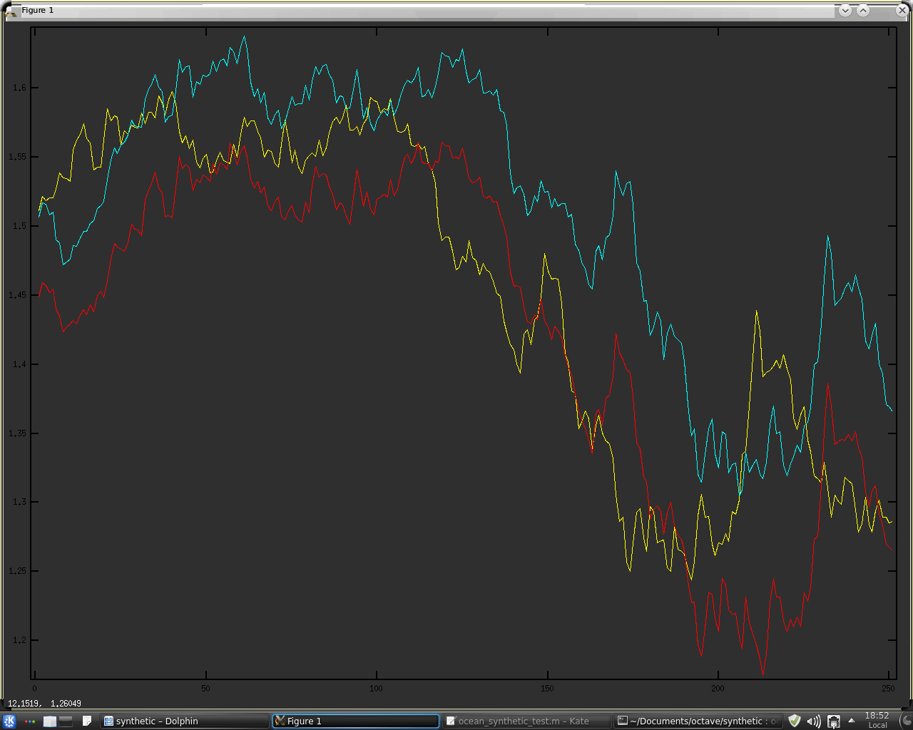
The last chart output of the script will look something like this.
The red sinusoid represents an underlying periodic signal of period 20 and the green time series is a composite signal of the red line plus a 7 period sinusoid of less amplitude and random noise, these not being shown in the plot. The blue line is the resultant output of FFT filtering in the frequency domain of the green input. I must say I'm pretty pleased with this result and will be doing more work in this area shortly. Stay tuned!