Expressing an Indicator in Neural Net Form

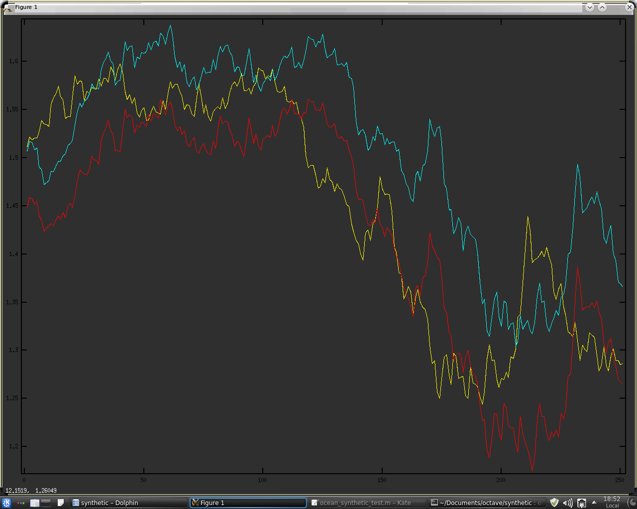
Recently I started investigating relative rotation graphs with a view to perhaps implementing a version of this for use on forex currency pairs. The underlying idea of a relative rotation graph is to plot an asset's relative strength compared to a benchmark and the momentum of this relative strength and to plot this in a form similar to a Polar coordinate system plot, which rotates around a zero point representing zero relative strength and zero relative strength momentum. After some thought it occurred to me that rather than using relative strength against a benchmark I could use the underlying relative strengths of the individual currencies, as calculated by my currency strength indicator, against each other. Furthermore, these underlying log changes in the individual currencies can be normalised using the ideas of brownian motion and then averaged together over different look back periods to create a unique indicator.

This indicator was coded up in the "traditional" way that will be familiar to anybody who has ever tried coding a trading indicator in any coding language. However, I thought that if the calculation of this indicator could be expressed in the form of a Feedforward neural network then the optimisation opportunities available using backpropagation and regularization could be used to tweek the indicator in more useful ways than just varying a look back length and amount of averaging. After some work I was able to make this work in just these two lines of Octave code:

indicator_middle_layer = tanh( full_feature_matrix * input_weights ) ;
indicator_nn_output = tanh( indicator_middle_layer * output_weights ) ; 

Of course, prior to calling these two lines of code, there is some feature engineering to create the input full_feature_matrix, and the input weights and output_weights matrices taken together are mathematically equivalent to the original indicator calculations. Finally, because this is a neural net expression of the indicator, the non-linear tanh activation function is applied to the hidden middle and output layers of the net.

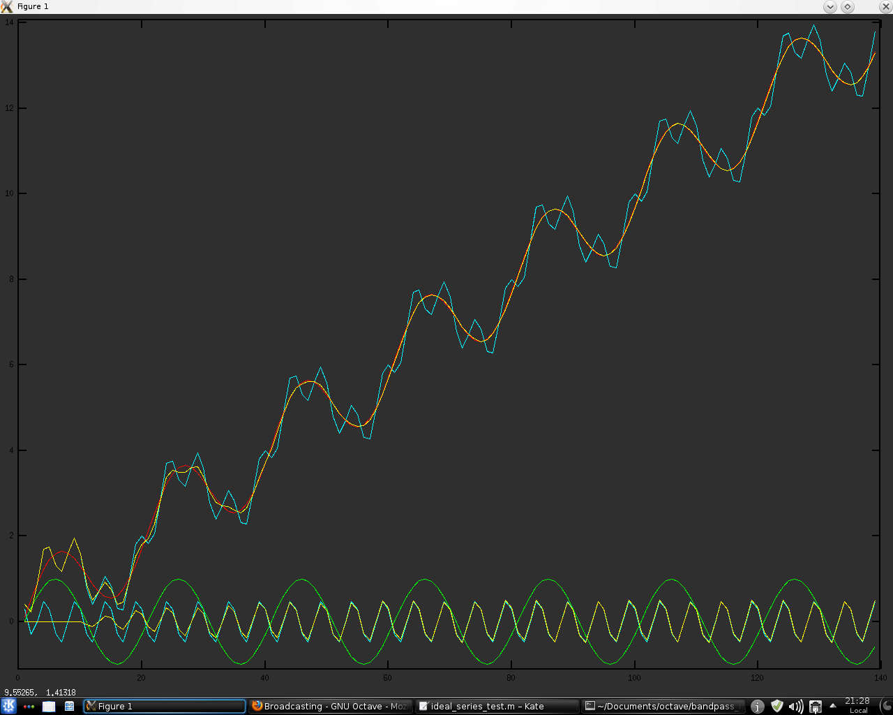
The following plot shows the original indicator in black and the neural net version of it in blue 

over the data shown in this plot of 10 minute bars of the EURUSD forex pair. 

The red indicator in the plot above is the 1 bar momentum of the neural net indicator plot.

To judge the quality of this indicator I used the entropy measure (measured over 14,000+ 10 minute bars of EURUSD), the results of which are shown next.

entropy_indicator_original = 0.9485
entropy_indicator_nn_output = 0.9933

An entropy reading of 0.9933 is probably as good as any trading indicator could hope to achieve (a perfect reading is 1.0) and so the next thing was to quickly back test the indicator performance. Based on the logic of the indicator the obvious long (short) signals are being above (below) the zeroline, or equivalently the sign of the indicator, and for good measure I also tested the sign of the momentum and some simple moving averages thereof.

The following plot shows the equity curves of this quick test where it is visually clear that the blue equity curves are "the best" when plotted in relation to the black "buy and hold" equivalent equity curve. These represent the equity curves of a 3 bar simple moving average of the 1 bar momentum of both the original formulation of the indicator and the neural net implementation. I would point out that these equity curves represent the theoretical equity resulting from trading the London session after 9:00am BST and stopping at 7:00am EST (usually about noon BST) and then starting trading again at 9:00am EST until 17:00pm EST. This schedule avoids the opening sessions (7:00 to 9:00am) in both London and New York because, from my observations of many OHLC charts such as shown above, there are frequently wild swings where price is being pushed to significant points such as volume profile clusters, accumulations of buy/sell orders etc. and in my opinion no indicator can be expected to perform well in that sort of environment. Also avoided are the hours prior to 7:00am BST, i.e. the Asian session or overnight session.    

Although these equity curves might not, at first glance, be that impressive, especially as they do not account for trading costs etc. my intent on doing these tests was to determine the configuration of a final "decision" output layer to be added to the neural net implementation of the indicator. A 3 bar simple moving average of the 1 bar momentum implies the necessity to include 4 consecutive readings of the indicator output as input to a final " decision" layer. The following simple, hand-drawn sketch shows what I mean:

A discussion of this will be the subject of my next post.

Simple Machine Learning Models on OrderBook/PositionBook Features

This post is about using OrderBook/PositionBook features as input to simple machine learning models after previous investigation into the relevance of such features. 

Due to the amount of training data available I decided to look only at a linear model and small neural networks (NN) with a single hidden layer with up to 6 hidden neurons. This choice was motivated by an academic paper I read online about linear models which stated that, as a lower bound, one should have at least 10 training examples for each parameter to be estimated. Other online reading about order flow imbalance (OFI) suggested there is a linear relationship between OFI and price movement. Use of limited size NNs would allow a small amount of non linearity in the relationship. For this investigation I used the Netlab toolbox and Octave. A plot of the learning curves of the classification models tested is shown below. The targets were binary 1/0 for price increases/decreases.

The blue lines show the average training error (y axis) and the red lines show the same average error metric on the held out cross validation data set for each tested model. The thickness of the lines represents the number of neurons in the single hidden layer of the NNs (the thicker the lines, the higher the number of hidden neurons). The horizontal green line shows the error of a generalized linear model (GLM) trained using iteratively reweighted least squares. It can be seen that NN models with 1 and 2 hidden neurons slightly outperform the GLM, with the 2 neuron model having the edge over the 1 neuron model. NN models with 3 or more hidden neurons over fit and underperform the GLM. The NN models were trained using Netlab's functions for Bayesian regularization over the parameters.

Looking at these results it would seem that a 2 neuron NN would be the best choice; however the error differences between the 1 and 2 neuron NNs and GLM are small enough to anticipate that the final classifications (with a basic greater/less than a 0.5 logistic threshold value for long/short) would perhaps be almost identical. 

Investigations into this will be the subject of my next post. 

The code box below gives the working Octave code for the above.

## load data
##training_data = dlmread( 'raw_netlab_training_features' ) ;
##cv_data = dlmread( 'raw_netlab_cv_features' ) ;
training_data = dlmread( 'netlab_training_features_svd' ) ;
cv_data = dlmread( 'netlab_cv_features_svd' ) ;
training_targets = dlmread( 'netlab_training_targets' ) ;
cv_targets = dlmread( 'netlab_cv_targets' ) ;

kk_loop_record = zeros( 30 , 7 ) ;

for kk = 1 : 30
  
## first train a glm model as a base comparison
input_dim = size( training_data , 2 ) ; ## Number of inputs.

net_lin = glm( input_dim , 1 , 'logistic' ) ; ## Create a generalized linear model structure.
options = foptions ; ## Sets default parameters for optimisation routines, for compatibility with MATLAB's foptions()
options(1) = 1 ;  ## change default value
##	OPTIONS(1) is set to 1 to display error values during training. If
##	OPTIONS(1) is set to 0, then only warning messages are displayed.  If
##	OPTIONS(1) is -1, then nothing is displayed.
options(14) = 5 ; ## change default value
##	OPTIONS(14) is the maximum number of iterations for the IRLS
##	algorithm;  default 100.
net_lin = glmtrain( net_lin , options , training_data , training_targets ) ;

## test on cv_data
glm_out = glmfwd( net_lin , cv_data ) ;
## cross-entrophy loss
glm_out_loss = -mean( cv_targets .* log( glm_out )  .+ ( 1 .- cv_targets ) .* log( 1 .- glm_out ) ) ;

kk_loop_record( kk , 7 ) = glm_out_loss ;

## now train an mlp
## Set up vector of options for the optimiser.
nouter = 30 ; ## Number of outer loops.
ninner = 2 ;	## Number of innter loops.
options = foptions ; ## Default options vector.
options( 1 ) = 1 ;	## This provides display of error values.
options( 2 ) = 1.0e-5 ; ## Absolute precision for weights.
options( 3 ) = 1.0e-5 ; ## Precision for objective function.
options( 14 ) = 100 ; ## Number of training cycles in inner loop.

training_learning_curve = zeros( nouter , 6 ) ; 
cv_learning_curve = zeros( nouter , 6 ) ;

for jj = 1 : 6

## Set up network parameters.
nin = size( training_data , 2 ) ; ## Number of inputs.
nhidden = jj ;	## Number of hidden units.
nout = 1 ; ## Number of outputs.
alpha = 0.01 ; ## Initial prior hyperparameter.
aw1 = 0.01 ;
ab1 = 0.01 ;
aw2 = 0.01 ;
ab2 = 0.01 ;

## Create and initialize network weight vector.
prior = mlpprior(nin , nhidden , nout , aw1 , ab1 , aw2 , ab2 ) ;
net = mlp( nin , nhidden , nout , 'logistic' , prior ) ;

## Train using scaled conjugate gradients, re-estimating alpha and beta.
for ii = 1 : nouter
  ## train net
  net = netopt( net , options , training_data , training_targets , 'scg' ) ;
  
  train_out = mlpfwd( net , training_data ) ;
  ## get train error
  ## mse
  ##training_learning_curve( ii ) = mean( ( training_targets .- train_out ).^2 ) ;
  
  ## cross entropy loss
  training_learning_curve( ii , jj ) = -mean( training_targets .* log( train_out )  .+ ( 1 .- training_targets ) .* log( 1 .- train_out ) ) ; 

  cv_out = mlpfwd( net , cv_data ) ;
  ## get cv error
  ## mse
  ##cv_learning_curve( ii ) = mean( ( cv_targets .- cv_out ).^2 ) ;
  
  ## cross entropy loss
  cv_learning_curve( ii , jj ) = -mean( cv_targets .* log( cv_out )  .+ ( 1 .- cv_targets ) .* log( 1 .- cv_out ) ) ; 
  
  ## now update hyperparameters based on evidence
  [ net , gamma ] = evidence( net , training_data , training_targets , ninner ) ;
  
##  fprintf( 1 , '\nRe-estimation cycle ##d:\n' , ii ) ;
##  disp( [ '  alpha = ' , num2str( net.alpha' ) ] ) ;
##  fprintf( 1 , '  gamma =  %8.5f\n\n' , gamma ) ;
##  disp(' ')
##  disp('Press any key to continue.')
  ##pause;
endfor ## ii loop

endfor ## jj loop

kk_loop_record( kk , 1 : 6 ) = cv_learning_curve( end , : ) ;

endfor ## kk loop

plot( training_learning_curve(:,1) , 'b' , 'linewidth' , 1 , cv_learning_curve(:,1) , 'r' , 'linewidth' , 1 , ...
training_learning_curve(:,2) , 'b' , 'linewidth' , 2 , cv_learning_curve(:,2) , 'r' , 'linewidth' , 2 , ...
training_learning_curve(:,3) , 'b' , 'linewidth' , 3 , cv_learning_curve(:,3) , 'r' , 'linewidth' , 3 , ...
training_learning_curve(:,4) , 'b' , 'linewidth' , 4 , cv_learning_curve(:,4) , 'r' , 'linewidth' , 4 , ...
training_learning_curve(:,5) , 'b' , 'linewidth' , 5 , cv_learning_curve(:,5) , 'r' , 'linewidth' , 5 , ...
training_learning_curve(:,6) , 'b' , 'linewidth' , 6 , cv_learning_curve(:,6) , 'r' , 'linewidth' , 6 , ...
ones( size( training_learning_curve , 1 ) , 1 ).*glm_out_loss , 'g' , 'linewidth', 2 ) ;

##  >> mean(kk_loop_record)
##  ans =
##
##     0.6928   0.6927   0.7261   0.7509   0.7821   0.8112   0.6990

##  >> std(kk_loop_record)
##  ans =
##
##     8.5241e-06   7.2869e-06   1.2999e-02   1.5285e-02   2.5769e-02   2.6844e-02   2.2584e-16

The Ideal Tau for Time Series Embedding?

In my Preliminary Test Results of Time Series Embedding post I got a bit ahead of myself and mistakenly quoted the ideal embedding length (Tau) to be half a period for cyclic prices. This should actually have been a quarter of a period and I have now corrected my earlier post.

This post is about my further investigations, which uncovered the above, and is written in a logical progression rather than the order in which I actually did things.

It was important to look at the Tau value for ideal sinusoidal data to confirm the quarter period, which checked out because I was able to easily recreate the 2D Lissajous curves in the Novel Method for Topological Embedding of Time-Series Data paper. I then extended this approach to 3D to produce plots such as this one, which may require some explaining.

This is a 3D Phase space plot of adaptive Max Min Normalised "sinusoidal prices" normalised to fall in the range [ -1 +1 ] and adaptive to the known, underlying period of the sine wave. This was done for prices with and without a "trend." The circular orbits are for the pure sine wave, representing cyclic price action plotted in 3D as current price, price delayed by a quarter of a cycle (Tau 1) and by half a cycle (Tau 2). The mini, blue and red "constellations" outside the circular orbits are the same pure sine wave(s) with an uptrend and downtrend added. The utility of this representation for market classification etc. is obvious, but is not the focus of this post.

Looking at Tau values for ideal prices with various trends taken from real market data, normalised as described above, across a range of known periods (because they were synthetically generated) the following results were obtained.

This is a plot of periods 10 to 47 (left to right along the x-axis) vs the global tau value (y-axis) measured using my Octave version of the mdDelay.m function from the mdembedding github. Each individual, coloured line plot is based on the underlying trend of one of 66 different, real time series. Each point per period per tradeable is the median value of 20 Monte Carlo runs over that tradeable's trend + synthetic, ideal sine wave price. The thick, black line is the median of the median values per period. Although noisy, it can be seen that the median line(s) straddle the theoretical, quarter cycle Tau (0.25) quite nicely. It should be remembered that this is on normalised prices. For comparison, the below plot shows the same on the unnormalised prices.

where the Tau value starts at over 0.5 at a cyclic period of 10 at the left and then slowly decreases to just over 0.1 at period 47.

More in due course.

Time Warp Edit Distance

Part of my normal routine is to indulge in online research for use useful ideas, and I recently came across An Empirical Evaluation of Similarity Measures for Time Series Classification, and one standout from this paper is the Time Warp Edit Distance where, from the conclusion, "...the TWED measure originally proposed by Marteau (2009) seems to consistently outperform all the considered distances..."

Below is my Octave .oct function version of the above linked MATLAB code.

#include octave oct.h
#include octave dmatrix.h
#include limits> // for infinity
#include math.h  // for sqrt

DEFUN_DLD ( twed, args, nargout,
"-*- texinfo -*-\n\
@deftypefn {Function File} {} twed (@var{A , timeSA , B , timeSB , lambda, nu})\n\
Calculates the Time Warp Edit Distance between two univariate time series, A and B.\n\
timeSA and timeSB are the time stamps of the respective series, lambda is a penalty\n\
for a deletion operation and nu is an Elasticity parameter - nu >=0 needed for distance measure.\n\
@end deftypefn" )

{
octave_value_list retval_list ;
int nargin = args.length () ;

// check the input arguments
if ( nargin != 6 )
   {
   error ("Invalid number of arguments. See help twed.") ;
   return retval_list ;
   }

if ( args(0).length () < 2 )
   {
   error ("Invalid 1st argument length. Must be >= 2.") ;
   return retval_list ;
   }
   
if ( args(1).length () != args(0).length () )
   {
   error ("Arguments 1 and 2 must be vectors of the same length.") ;
   return retval_list ;
   }
   
if ( args(2).length () < 2 )
   {
   error ("Invalid 3rd argument length. Must be >= 2.") ;
   return retval_list ;
   }
   
if ( args(3).length () != args(2).length () )
   {
   error ("Arguments 3 and 4 must be vectors of the same length.") ;
   return retval_list ;
   }   
   
if ( args(4).length () > 1 )
   {
   error ("Argument 5 must a single value for lambda.") ;
   return retval_list ;
   }  
  
if ( args(5).length () > 1 )
   {
   error ("Argument 6 must a single value for nu >= 0.") ;
   return retval_list ;
   }   

if ( error_state )
   {
   error ("Invalid arguments. See help twed.") ;
   return retval_list ;
   }
// end of input checking  
  
Matrix A_input = args(0).matrix_value () ;
   if( A_input.rows() == 1 && A_input.cols() >= 2 ) // is a row matrix, so transpose 
   {
    A_input = A_input.transpose () ; 
   }
   
Matrix timeSA_input = args(1).matrix_value () ;
   if( timeSA_input.rows() == 1 && timeSA_input.cols() >= 2 ) // is a row matrix, so transpose 
   {
    timeSA_input = timeSA_input.transpose () ; 
   }
   
Matrix B_input = args(2).matrix_value () ;
   if( B_input.rows() == 1 && B_input.cols() >= 2 ) // is a row matrix, so transpose 
   {
    B_input = B_input.transpose () ; 
   }
   
Matrix timeSB_input = args(3).matrix_value () ;
   if( timeSB_input.rows() == 1 && timeSB_input.cols() >= 2 ) // is a row matrix, so transpose 
   {
    timeSB_input = timeSB_input.transpose () ; 
   }
   
double lambda = args(4).double_value () ;
double nu = args(5).double_value () ;
double inf = std::numeric_limits::infinity() ;
Matrix distance ( 1 , 1 ) ; distance.fill ( 0.0 ) ;
double cost ;
  
// Add padding of zero by using zero-filled distance matrix
Matrix A = distance.stack( A_input ) ;
Matrix timeSA = distance.stack( timeSA_input ) ;
Matrix B = distance.stack( B_input ) ;
Matrix timeSB = distance.stack( timeSB_input ) ;

Matrix DP ( A.rows() , B.rows() ) ; DP.fill ( inf ) ; DP( 0 , 0 ) = 0.0 ; 
int n = timeSA.rows () ;
int m = timeSB.rows () ;

    // Compute minimal cost
    for ( octave_idx_type ii (1) ; ii < n ; ii++ )
    {
      
        for ( octave_idx_type jj (1) ; jj < m ; jj++ )
        {
          
        // Deletion in A
        DP( ii , jj ) = DP(ii-1,jj) +  sqrt( ( A(ii-1,0) - A(ii,0) ) * ( A(ii-1,0) - A(ii,0) ) ) + nu * ( timeSA(ii,0) - timeSA(ii-1,0) ) + lambda ;
    
        // Deletion in B
        cost = DP(ii,jj-1) + sqrt( ( B(jj-1,0) - B(jj,0) ) * ( B(jj-1,0) - B(jj,0) ) ) + nu * ( timeSB(jj,0) - timeSB(jj-1,0) ) + lambda ;
        DP( ii , jj ) = cost < DP( ii , jj ) ? cost : DP( ii , jj ) ;
    
        // Keep data points in both time series
        cost = DP(ii-1,jj-1) + sqrt( ( A(ii,0) - B(jj,0) ) * ( A(ii,0) - B(jj,0) ) ) + sqrt( ( A(ii-1,0) - B(jj-1,0) ) * ( A(ii-1,0) - B(jj-1,0) ) ) + nu * ( abs( timeSA(ii,0) - timeSB(jj,0) ) + abs( timeSA(ii-1,0) - timeSB(jj-1,0) ) ) ;
        DP( ii , jj ) = cost < DP( ii , jj ) ? cost : DP( ii , jj ) ;

        } // end of jj loop
        
      } // end of ii loop

distance( 0 , 0 ) = DP( n - 1 , m - 1 ) ;
      
retval_list(1) = DP ; 
retval_list(0) = distance ;

return retval_list ;

} // end of function

As a quick test I took the example problem from this Cross Validated thread, the applicability I hope being quite obvious to readers:

A = [1, 2, 3, 4, 5, 6, 7, 8, 9] ;
B1 = [1, 2, 3, 4, 5, 6, 7, 8, 12] ;
distance1 = twed( A , 1:9 , B1 , 1:9 , 1 , 0.001 )
distance1 =  3
B2 = [0, 3, 2, 5, 4, 7, 6, 9, 8] ;
distance2 = twed( A , 1:9 , B2 , 1:9 , 1 , 0.001 )
distance2 =  17
graphics_toolkit('fltk') ; plot(A,'k','linewidth',2,B1,'b','linewidth',2,B2,'r','linewidth',2);
legend( "A" , "B1" , "B2" ) ;

It can be seen that the twed algorithm correctly picks out B1 as being more like A than B2 (a lower twed distance, with default values for lambda and nu of 1 and 0.001 respectively, taken from the above survey paper) when compared with the simple squared error metric, which gives identical results for both B1 and B2.

More on this in due course.

Update on Recent Work

It has been almost two months since my last post and during this time I have been working on a few different things, all related in one way or another to my desire to create a rolling NN training regime. First off, I have been giving some thought as to the exact methodology to use, and two had come to mind

1. a rolling look back period of n bars, similar to a moving average
2. selecting non consecutive periods of price history with similarity to the most recent history

I have not done any work on the first because I feel that it might lead to an unbalanced training set, so I have been working on the second idea. It seemed natural to revisit my earlier work on market classifying with the idea of training a NN for the current market regime using the most recent n bars that have the same market regime classification as the current bar. However, having been somewhat disappointed with the results of my previous work in  this area I have been looking at SVM classifiers, in particular the libsvm library. To facilitate this, and following on from my previous post where I mentioned the comp engine timeseries website, I have been hand engineering features for inputs to the SVM. Below is a short video which shows the four features I have come up with. The x and y axis are the same two features in both parts of the video, with the z axis being the third and fourth features. The data are those obtained from my usual idealised market types, with added noise to try and simulate more realistic market conditions. The different colours indicate the five market types that are being modelled.

Non-embedded view

As can be seen there is nice separation between the market types and the SVM achieves over 98% cross-validation accuracy on this training set. Despite this,  when applied to real market data I am yet again disappointed by the performance and choose for now to no longer pursue this avenue of investigation.

In addition to all the above, I have "discovered" the Octave sourceforge nan package, which I may begin to investigate more fully in due course. I have also been working through another Massive Open Online Course, this time Statistical Learning, which is in its last week at the moment. In this last week of the course I have been alerted to a possible new area of investigation, Distance correlation, which I had heard of before but not fully appreciated.

Finally, I have also been reassessing the code I use for calculating dominant cycle periods. It is these last two, distance correlation and the period code, that I'm going to look at more fully over the coming days.

Brownian Bands

For the past few weeks I have been working on the idea presented in my earlier modelling prices using brownian motion post and below is a video of what I have come up with, which I'm calling Brownian Bands. The video shows these bands on the EURUSD forex pair with look back lengths of 1 to 10 bars inclusive, then 15 to 50 in increments of 5, then 50, 100 and 200 and finally 50, 100 and 200 on the whole time series. Each look back length band is the average of all bands from 1 up to and including the look back length band - the details of the implementation can be seen in the code boxes below. The blue band is the upper band, the red is the lower and the green is the mid point of the two.

           
Non-embedded view.

This following chart shows an adaptive look back length implementation, the look back length being determined by a period vector input to the function, which in this case is the dominant cycle period.

These adaptive Brownian bands can be compared with the equivalent adaptive Bollinger bands shown in this next chart.

For my intended purpose of separating out returns into distribution bins the Brownian bands seem to be superior. There are 3 distinct bins: above the upper band, below the lower band and between the bands, whereas with the Bollinger bands the vast majority of returns would be lumped into just one bin - between the bands. Of course the Brownian bands could be used to create a system indicator just as Bollinger bands can be, and if any readers test this idea I would be intrigued to hear of your results. However, should you choose to do this there is a major caveat you should be aware of. The calculation of the Brownian bands is based on the natural log of actual price, which means you should be very wary of test results on any back adjusted price series such as futures and adjusted stock prices. In fact I would go as far to say that the code given below should not be used as is on such price series. It is for this reason that I have been using forex price series in my own tests so far, but I will surely get around to adjusting the given code in due course.

Now for the code. This first code box shows a hard-coded, unrolled loop version for look back lengths up to and including 25 for the benefit of a reader who requested a clearer exposition of the method than was given in my earlier post, which was vectorised Octave code. All the code below is C++ as used in Octave .oct files.

DEFUN_DLD ( brownian_bands_25, args, nargout, 
"-*- texinfo -*-\n\
@deftypefn {Function File} {} brownian_bands_25 (@var{price,period})\n\
This function takes a price vector input and a value for the tick\n\
size of the instrument and outputs upper and lower bands based on\n\
the concept of Brownian motion. The bands are the average of look\n\
back periods of 1 to 25 bars inclusive of the relevant calculations.\n\
@end deftypefn" )

{
octave_value_list retval_list ;
int nargin = args.length () ;

// check the input arguments
if ( nargin != 2 )
   {
   error ( "Invalid arguments. Type help to see usage." ) ;
   return retval_list ;
   }

if ( args(0).length () < 21 )
   {
   error ( "Invalid arguments. Type help to see usage." ) ;
   return retval_list ;
   }
   
if ( args(1).length () != 1 )
   {
   error ( "Invalid arguments. Type help to see usage." ) ;
   return retval_list ;
   }   

if ( error_state )
   {
   error ( "Invalid arguments. Type help to see usage." ) ;
   return retval_list ;
   }
// end of input checking   

ColumnVector price = args(0).column_vector_value () ;
double tick_size = args(1).double_value() ;
ColumnVector abs_log_price_diff = args(0).column_vector_value () ;
ColumnVector upper_band = args(0).column_vector_value () ;
ColumnVector lower_band = args(0).column_vector_value () ;
ColumnVector mid_band = args(0).column_vector_value () ;
double sum ;

double up_1 ;
double low_1 ;

double up_2 ;
double low_2 ;
double sqrt_2 = sqrt(2.0) ; // pre-calculated for speed optimisation

double up_3 ;
double low_3 ;
double sqrt_3 = sqrt(3.0) ; // pre-calculated for speed optimisation

double up_4 ;
double low_4 ;
double sqrt_4 = sqrt(4.0) ; // pre-calculated for speed optimisation

double up_5 ;
double low_5 ;
double sqrt_5 = sqrt(5.0) ; // pre-calculated for speed optimisation

double up_6 ;
double low_6 ;
double sqrt_6 = sqrt(6.0) ; // pre-calculated for speed optimisation

double up_7 ;
double low_7 ;
double sqrt_7 = sqrt(7.0) ; // pre-calculated for speed optimisation

double up_8 ;
double low_8 ;
double sqrt_8 = sqrt(8.0) ; // pre-calculated for speed optimisation

double up_9 ;
double low_9 ;
double sqrt_9 = sqrt(9.0) ; // pre-calculated for speed optimisation

double up_10 ;
double low_10 ;
double sqrt_10 = sqrt(10.0) ; // pre-calculated for speed optimisation

double up_11 ;
double low_11 ;
double sqrt_11 = sqrt(11.0) ; // pre-calculated for speed optimisation

double up_12 ;
double low_12 ;
double sqrt_12 = sqrt(12.0) ; // pre-calculated for speed optimisation

double up_13 ;
double low_13 ;
double sqrt_13 = sqrt(13.0) ; // pre-calculated for speed optimisation

double up_14 ;
double low_14 ;
double sqrt_14 = sqrt(14.0) ; // pre-calculated for speed optimisation

double up_15 ;
double low_15 ;
double sqrt_15 = sqrt(15.0) ; // pre-calculated for speed optimisation

double up_16 ;
double low_16 ;
double sqrt_16 = sqrt(16.0) ; // pre-calculated for speed optimisation

double up_17 ;
double low_17 ;
double sqrt_17 = sqrt(17.0) ; // pre-calculated for speed optimisation

double up_18 ;
double low_18 ;
double sqrt_18 = sqrt(18.0) ; // pre-calculated for speed optimisation

double up_19 ;
double low_19 ;
double sqrt_19 = sqrt(19.0) ; // pre-calculated for speed optimisation

double up_20 ;
double low_20 ;
double sqrt_20 = sqrt(20.0) ; // pre-calculated for speed optimisation

double up_21 ;
double low_21 ;
double sqrt_21 = sqrt(21.0) ; // pre-calculated for speed optimisation

double up_22 ;
double low_22 ;
double sqrt_22 = sqrt(22.0) ; // pre-calculated for speed optimisation

double up_23 ;
double low_23 ;
double sqrt_23 = sqrt(23.0) ; // pre-calculated for speed optimisation

double up_24 ;
double low_24 ;
double sqrt_24 = sqrt(24.0) ; // pre-calculated for speed optimisation

double up_25 ;
double low_25 ;
double sqrt_25 = sqrt(25.0) ; // pre-calculated for speed optimisation

for ( octave_idx_type ii (1) ; ii < 25 ; ii++ ) // initialising loop 
    {
    abs_log_price_diff(ii) = fabs( log( price(ii) ) - log( price(ii-1) ) ) ;
    }
    
for ( octave_idx_type ii (25) ; ii < args(0).length () ; ii++ ) // main loop
    {
      
    abs_log_price_diff(ii) = fabs( log( price(ii) ) - log( price(ii-1) ) ) ;

    sum = abs_log_price_diff(ii) ;
    up_1 = exp( log( price(ii-1) ) + sum ) ;
    low_1 = exp( log( price(ii-1) ) - sum ) ;

    sum += abs_log_price_diff(ii-1) ;
    up_2 = exp( log( price(ii-2) ) + (sum/2.0) * sqrt_2 ) ;
    low_2 = exp( log( price(ii-2) ) - (sum/2.0) * sqrt_2 ) ;

    sum += abs_log_price_diff(ii-2) ;
    up_3 = exp( log( price(ii-3) ) + (sum/3.0) * sqrt_3 ) ;
    low_3 = exp( log( price(ii-3) ) - (sum/3.0) * sqrt_3 ) ;
    
    sum += abs_log_price_diff(ii-3) ;
    up_4 = exp( log( price(ii-4) ) + (sum/4.0) * sqrt_4 ) ;
    low_4 = exp( log( price(ii-4) ) - (sum/4.0) * sqrt_4 ) ;

    sum += abs_log_price_diff(ii-4) ;
    up_5 = exp( log( price(ii-5) ) + (sum/5.0) * sqrt_5 ) ;
    low_5 = exp( log( price(ii-5) ) - (sum/5.0) * sqrt_5 ) ;    

    sum += abs_log_price_diff(ii-5) ;
    up_6 = exp( log( price(ii-6) ) + (sum/6.0) * sqrt_6 ) ;
    low_6 = exp( log( price(ii-6) ) - (sum/6.0) * sqrt_6 ) ;
    
    sum += abs_log_price_diff(ii-6) ;
    up_7 = exp( log( price(ii-7) ) + (sum/7.0) * sqrt_7 ) ;
    low_7 = exp( log( price(ii-7) ) - (sum/7.0) * sqrt_7 ) ;
    
    sum += abs_log_price_diff(ii-7) ;
    up_8 = exp( log( price(ii-8) ) + (sum/8.0) * sqrt_8 ) ;
    low_8 = exp( log( price(ii-8) ) - (sum/8.0) * sqrt_8 ) ;
    
    sum += abs_log_price_diff(ii-8) ;
    up_9 = exp( log( price(ii-9) ) + (sum/9.0) * sqrt_9 ) ;
    low_9 = exp( log( price(ii-9) ) - (sum/9.0) * sqrt_9 ) ;
    
    sum += abs_log_price_diff(ii-9) ;
    up_10 = exp( log( price(ii-10) ) + (sum/10.0) * sqrt_10 ) ;
    low_10 = exp( log( price(ii-10) ) - (sum/10.0) * sqrt_10 ) ;
    
    sum += abs_log_price_diff(ii-10) ;
    up_11 = exp( log( price(ii-11) ) + (sum/11.0) * sqrt_11 ) ;
    low_11 = exp( log( price(ii-11) ) - (sum/11.0) * sqrt_11 ) ;
    
    sum += abs_log_price_diff(ii-11) ;
    up_12 = exp( log( price(ii-12) ) + (sum/12.0) * sqrt_12 ) ;
    low_12 = exp( log( price(ii-12) ) - (sum/12.0) * sqrt_12 ) ;
    
    sum += abs_log_price_diff(ii-12) ;
    up_13 = exp( log( price(ii-13) ) + (sum/13.0) * sqrt_13 ) ;
    low_13 = exp( log( price(ii-13) ) - (sum/13.0) * sqrt_13 ) ;
    
    sum += abs_log_price_diff(ii-13) ;
    up_14 = exp( log( price(ii-14) ) + (sum/14.0) * sqrt_14 ) ;
    low_14 = exp( log( price(ii-14) ) - (sum/14.0) * sqrt_14 ) ;
    
    sum += abs_log_price_diff(ii-14) ;
    up_15 = exp( log( price(ii-15) ) + (sum/15.0) * sqrt_15 ) ;
    low_15 = exp( log( price(ii-15) ) - (sum/15.0) * sqrt_15 ) ;
    
    sum += abs_log_price_diff(ii-15) ;
    up_16 = exp( log( price(ii-16) ) + (sum/16.0) * sqrt_16 ) ;
    low_16 = exp( log( price(ii-16) ) - (sum/16.0) * sqrt_16 ) ;
    
    sum += abs_log_price_diff(ii-16) ;
    up_17 = exp( log( price(ii-17) ) + (sum/17.0) * sqrt_17 ) ;
    low_17 = exp( log( price(ii-17) ) - (sum/17.0) * sqrt_17 ) ;
    
    sum += abs_log_price_diff(ii-17) ;
    up_18 = exp( log( price(ii-18) ) + (sum/18.0) * sqrt_18 ) ;
    low_18 = exp( log( price(ii-18) ) - (sum/18.0) * sqrt_18 ) ;
    
    sum += abs_log_price_diff(ii-18) ;
    up_19 = exp( log( price(ii-19) ) + (sum/19.0) * sqrt_19 ) ;
    low_19 = exp( log( price(ii-19) ) - (sum/19.0) * sqrt_19 ) ;
    
    sum += abs_log_price_diff(ii-19) ;
    up_20 = exp( log( price(ii-20) ) + (sum/20.0) * sqrt_20 ) ;
    low_20 = exp( log( price(ii-20) ) - (sum/20.0) * sqrt_20 ) ;
    
    sum += abs_log_price_diff(ii-20) ;
    up_21 = exp( log( price(ii-21) ) + (sum/21.0) * sqrt_21 ) ;
    low_21 = exp( log( price(ii-21) ) - (sum/21.0) * sqrt_21 ) ;
    
    sum += abs_log_price_diff(ii-21) ;
    up_22 = exp( log( price(ii-22) ) + (sum/22.0) * sqrt_22 ) ;
    low_22 = exp( log( price(ii-22) ) - (sum/22.0) * sqrt_22 ) ;
    
    sum += abs_log_price_diff(ii-22) ;
    up_23 = exp( log( price(ii-23) ) + (sum/23.0) * sqrt_23 ) ;
    low_23 = exp( log( price(ii-23) ) - (sum/23.0) * sqrt_23 ) ;
    
    sum += abs_log_price_diff(ii-23) ;
    up_24 = exp( log( price(ii-24) ) + (sum/24.0) * sqrt_24 ) ;
    low_24 = exp( log( price(ii-24) ) - (sum/24.0) * sqrt_24 ) ;
    
    sum += abs_log_price_diff(ii-24) ;
    up_25 = exp( log( price(ii-25) ) + (sum/25.0) * sqrt_25 ) ;
    low_25 = exp( log( price(ii-25) ) - (sum/25.0) * sqrt_25 ) ;
    
    upper_band(ii) = (up_1+up_2+up_3+up_4+up_5+up_6+up_7+up_8+up_9+up_10+up_11+up_12+up_13+up_14+up_15+up_16+up_17+up_18+up_19+up_20+up_21+up_22+up_23+up_24+up_25)/25.0 ;
    lower_band(ii) = (low_1+low_2+low_3+low_4+low_5+low_6+low_7+low_8+low_9+low_10+low_11+low_12+low_13+low_14+low_15+low_16+low_17+low_18+low_19+low_20+low_21+low_22+low_23+up_24+low_25)/25.0 ;
    
    // round the upper_band up to the nearest tick
    upper_band(ii) = ceil( upper_band(ii)/tick_size ) * tick_size ;
    
    // round the lower_band down to the nearest tick
    lower_band(ii) = floor( lower_band(ii)/tick_size ) * tick_size ;
    
    mid_band(ii) = ( upper_band(ii) + lower_band(ii) ) / 2.0 ;
    
    } // end of main loop   

    retval_list(2) = mid_band ;
    retval_list(1) = lower_band ;
    retval_list(0) = upper_band ;

return retval_list ;

} // end of function

This next code box contains code for an adjustable look back length, the length being a user input to the function. This code wraps the above unrolled loop into a nested loop.

DEFUN_DLD ( brownian_bands_adjustable, args, nargout, 
"-*- texinfo -*-\n\
@deftypefn {Function File} {} brownian_bands_adjustable (@var{price,lookback,tick_size})\n\
This function takes a price vector input, a value for the lookback\n\
length and a value for the tick size of the instrument and outputs\n\
upper and lower bands based on the concept of Brownian motion. The bands\n\
are the average of lookback period bands from 1 to lookback length.\n\
@end deftypefn" )

{
octave_value_list retval_list ;
int nargin = args.length () ;

// check the input arguments
if ( nargin != 3 )
   {
   error ( "Invalid arguments. Type help to see usage." ) ;
   return retval_list ;
   }
   
if ( args(1).length () != 1 ) // lookback length argument
   {
   error ( "Invalid arguments. Type help to see usage." ) ;
   return retval_list ;
   }
   
double lookback = args(1).double_value() ;   

if ( args(0).length () < lookback ) // check length of price vector input
   {
   error ( "Invalid arguments. Type help to see usage." ) ;
   return retval_list ;
   }
   
if ( args(2).length () != 1 ) // tick size
   {
   error ( "Invalid arguments. Type help to see usage." ) ;
   return retval_list ;
   }   
   
if ( error_state )
   {
   error ( "Invalid arguments. Type help to see usage." ) ;
   return retval_list ;
   }
// end of input checking   

ColumnVector price = args(0).column_vector_value () ;
double tick_size = args(2).double_value() ;
ColumnVector abs_log_price_diff = args(0).column_vector_value () ;
ColumnVector upper_band = args(0).column_vector_value () ;
ColumnVector lower_band = args(0).column_vector_value () ;
ColumnVector mid_band = args(0).column_vector_value () ;
double sum ;
double up_bb ;
double low_bb ;
int jj ;

for ( octave_idx_type ii (1) ; ii < lookback ; ii++ ) // initialising loop 
    {
    abs_log_price_diff(ii) = fabs( log( price(ii) ) - log( price(ii-1) ) ) ;
    }
    
for ( octave_idx_type ii (lookback) ; ii < args(0).length () ; ii++ ) // main loop
    {    
    // initialise calculation values  
    sum = 0.0 ;
    up_bb = 0.0 ;
    low_bb = 0.0 ;

    for ( jj = 1 ; jj < lookback + 1 ; jj++ ) // nested jj loop
        {
   
 abs_log_price_diff(ii) = fabs( log( price(ii) ) - log( price(ii-1) ) ) ;
        sum += abs_log_price_diff(ii-jj+1) ;
        up_bb += exp( log( price(ii-jj) ) + (sum/double(jj)) * sqrt(double(jj)) ) ;
        low_bb += exp( log( price(ii-jj) ) - (sum/double(jj)) * sqrt(double(jj)) ) ;  

 } // end of nested jj loop  
    
    upper_band(ii) = up_bb / lookback ;
    lower_band(ii) = low_bb / lookback ;
    
    // round the upper_band up to the nearest tick
    upper_band(ii) = ceil( upper_band(ii)/tick_size ) * tick_size ;
    
    // round the lower_band down to the nearest tick
    lower_band(ii) = floor( lower_band(ii)/tick_size ) * tick_size ;
    
    mid_band(ii) = ( upper_band(ii) + lower_band(ii) ) / 2.0 ;
    
    } // end of main loop   

    retval_list(2) = mid_band ;
    retval_list(1) = lower_band ;
    retval_list(0) = upper_band ;

return retval_list ;

} // end of function

Finally, this code is the adaptive look back version where the length of the look back is contained in a vector which is also a user input.

DEFUN_DLD ( brownian_bands_adaptive, args, nargout, 
"-*- texinfo -*-\n\
@deftypefn {Function File} {} brownian_bands_adaptive (@var{price,period,tick_size})\n\
This function takes price and period vector inputs & a value for the tick\n\
size of the instrument and outputs upper and lower bands based on\n\
the concept of Brownian motion. The bands are adaptive averages of look\n\
back lengths of 1 to period bars inclusive.\n\
@end deftypefn" )

{
octave_value_list retval_list ;
int nargin = args.length () ;

// check the input arguments
if ( nargin != 3 )
   {
   error ( "Invalid arguments. Type help to see usage." ) ;
   return retval_list ;
   }
   
if ( args(0).length () < 50 ) // check length of price vector input
   {
   error ( "Invalid arguments. Type help to see usage." ) ;
   return retval_list ;
   }   
   
if ( args(1).length () != args(0).length () ) // lookback period length argument
   {
   error ( "Invalid arguments. Type help to see usage." ) ;
   return retval_list ;
   }
      
if ( args(2).length () != 1 ) // tick size
   {
   error ( "Invalid arguments. Type help to see usage." ) ;
   return retval_list ;
   }   
   
if ( error_state )
   {
   error ( "Invalid arguments. Type help to see usage." ) ;
   return retval_list ;
   }
// end of input checking   

ColumnVector price = args(0).column_vector_value () ;
ColumnVector period = args(1).column_vector_value () ; 
double tick_size = args(2).double_value() ;
ColumnVector abs_log_price_diff = args(0).column_vector_value () ;
ColumnVector upper_band = args(0).column_vector_value () ;
ColumnVector lower_band = args(0).column_vector_value () ;
ColumnVector mid_band = args(0).column_vector_value () ;
double sum ;
double up_bb ;
double low_bb ;
int jj ;

for ( octave_idx_type ii (1) ; ii < 50 ; ii++ ) // initialising loop 
    {
    abs_log_price_diff(ii) = fabs( log( price(ii) ) - log( price(ii-1) ) ) ;
    }
    
for ( octave_idx_type ii (50) ; ii < args(0).length () ; ii++ ) // main loop
    {    
    // initialise calculation values  
    sum = 0.0 ;
    up_bb = 0.0 ;
    low_bb = 0.0 ;

    for ( jj = 1 ; jj < period(ii) + 1 ; jj++ ) // nested jj loop
        {
   
 abs_log_price_diff(ii) = fabs( log( price(ii) ) - log( price(ii-1) ) ) ;
        sum += abs_log_price_diff(ii-jj+1) ;
        up_bb += exp( log( price(ii-jj) ) + (sum/double(jj)) * sqrt(double(jj)) ) ;
        low_bb += exp( log( price(ii-jj) ) - (sum/double(jj)) * sqrt(double(jj)) ) ;  

 } // end of nested jj loop  
    
    upper_band(ii) = up_bb / period(ii) ;
    lower_band(ii) = low_bb / period(ii) ;
    
    // round the upper_band up to the nearest tick
    upper_band(ii) = ceil( upper_band(ii)/tick_size ) * tick_size ;
    
    // round the lower_band down to the nearest tick
    lower_band(ii) = floor( lower_band(ii)/tick_size ) * tick_size ;
    
    mid_band(ii) = ( upper_band(ii) + lower_band(ii) ) / 2.0 ;
    
    } // end of main loop   

    retval_list(2) = mid_band ;
    retval_list(1) = lower_band ;
    retval_list(0) = upper_band ;

return retval_list ;

} // end of function

Due to formatting issues on Blogger none of the code boxes contain the required header statements, which should be:-

#include octave/oct.h
#include octave/dColVector.h
#include math.h

with the customary < before "octave" and "math" and > after ".h"

Exploratory Data Analysis of Brownian Motion Model

For my first steps in investigating the earlier proposed Brownian motion model I thought I would use some Exploratory Data Analysis techniques. I have initially decided to use look back periods of 5 bars and 21 bars; the 5 bar on daily data being a crude attempt to capture the essence of weekly price movement and the 21 bar to capture the majority of dominant cycle periods in daily data, with both parameters also being non optimised Fibonacci numbers. Using the two channels over price bars that these create it is possible to postulate nine separate and distinct price "regimes" using combinations of the criteria of being above, within or below each channel.

The use of these "regimes" is to bin normalised price change at time t into nine separate distributions, the normalising factor being the 5 bar simple moving average of absolute natural log differences at time t-1 and the choice of regime being determined by the position of the close at t-1. The rationale behind basing these metrics on preceding bars is explained in this earlier post and the implementation made clear in the code box at the end of this post. The following 4 charts are Box plots of these nine distributions, in consecutive order, for the EURUSD, GBPUSD, USDCHF and USDYEN  forex pairs:

Looking at these, I'm struck by two things. Firstly, the middle three box plots are for regimes where price is in the 21 bar channel, and numbering from the left, boxes 4, 5 and 6 are below the 5 bar channel, in it and above it. These are essentially different degrees of a sideways market and it can be seen that there are far more outliers here than in the other box plots, perhaps indicating the tendency for high volatility breakouts to occur more frequently in sideways markets.

The second thing that is striking is, again numbering from the left, box plots 3 and 7. These are regimes below the 21 bar and above the 5 bar; and above the 21 bar and below the 5 bar - essentially the distributions for reactions against prevailing trends on the 21 bar time scale. Here it can be seen that there are far fewer outliers and generally shorter whiskers, indicating the tendency for reactions against trends to be less volatile in nature.

It is encouraging to see that there are such differences in these box plots as it suggests that my idea of binning does separate out the different price change characteristics. However, I believe things can be improved a bit in this regard and this will form the subject matter of my next post.

clear all

data = load("-ascii","usdyen") ;
close = data(:,7) ;
logdiff = [ 0 ; diff( log(close) ) ] ;
abslogdiff = abs( logdiff ) ;

sq_rt = sqrt( 5 ) ;
sma5 = sma(abslogdiff,5) ;
ub5 = exp(shift(log(close),5).+(sma5.*sq_rt)) ;
lb5 = exp(shift(log(close),5).-(sma5.*sq_rt)) ;

sq_rt = sqrt( 21 ) ;
sma21 = sma(abslogdiff,21) ;
ub21 = exp(shift(log(close),21).+(sma21.*sq_rt)) ;
lb21 = exp(shift(log(close),21).-(sma21.*sq_rt)) ;

% allocate close bar to a market_type
market_type = zeros( size(close,1) , 1 ) ;

% above ub21 **********************
val_1 = close > ub21 ;
val_2 = close > ub5 ;
matches = val_1 .* val_2 ;
ix = find( matches == 1 ) ;
market_type( ix , 1 ) = 4 ;

val_1 = close > ub21 ;
val_2 = close <= ub5 ;
val_3 = close >= lb5 ;
matches = val_1 .* val_2 .* val_3 ;
ix = find( matches == 1 ) ;
market_type( ix , 1 ) = 3 ;

val_1 = close > ub21 ;
val_2 = close < lb5 ;
matches = val_1 .* val_2 ;
ix = find( matches == 1 ) ;
market_type( ix , 1 ) = 2 ;
%**********************************

% below lb21 **********************
val_1 = close < lb21 ;
val_2 = close < lb5 ;
matches = val_1 .* val_2 ;
ix = find( matches == 1 ) ;
market_type( ix , 1 ) = -4 ;

val_1 = close < lb21 ;
val_2 = close <= ub5 ;
val_3 = close >= lb5 ;
matches = val_1 .* val_2 .* val_3 ;
ix = find( matches == 1 ) ;
market_type( ix , 1 ) = -3 ;

val_1 = close < lb21 ;
val_2 = close > ub5 ;
matches = val_1 .* val_2 ;
ix = find( matches == 1 ) ;
market_type( ix , 1 ) = -2 ;
%**********************************

% between ub21 & lb21**************
val_1 = close <= ub21 ;
val_2 = close >= lb21 ;
val_3 = close > ub5 ;
matches = val_1 .* val_2 .* val_3 ;
ix = find( matches == 1 ) ;
market_type( ix , 1 ) = 1 ;

val_1 = close <= ub21 ;
val_2 = close >= lb21 ;
val_3 = close < lb5 ;
matches = val_1 .* val_2 .* val_3 ;
ix = find( matches == 1 ) ;
market_type( ix , 1 ) = -1 ;
%**********************************

% now allocate to bins
normalised_logdiffs = logdiff ./ shift( sma5 , 1 ) ;

% shift market_type to agree with normalised_logdiffs
shifted_market_type = shift( market_type , 1 ) ;

bin_4 = normalised_logdiffs( find( shifted_market_type(30:end,1) == 4 ) , 1 ) ;
bin_3 = normalised_logdiffs( find( shifted_market_type(30:end,1) == 3 ) , 1 ) ;
bin_2 = normalised_logdiffs( find( shifted_market_type(30:end,1) == 2 ) , 1 ) ;
bin_1 = normalised_logdiffs( find( shifted_market_type(30:end,1) == 1 ) , 1 ) ;
bin_0 = normalised_logdiffs( find( shifted_market_type(30:end,1) == 0 ) , 1 ) ;
bin_1m = normalised_logdiffs( find( shifted_market_type(30:end,1) == -1 ) , 1 ) ;
bin_2m = normalised_logdiffs( find( shifted_market_type(30:end,1) == -2 ) , 1 ) ;
bin_3m = normalised_logdiffs( find( shifted_market_type(30:end,1) == -3 ) , 1 ) ;
bin_4m = normalised_logdiffs( find( shifted_market_type(30:end,1) == -4 ) , 1 ) ;

y_axis_max = max( normalised_logdiffs(30:end,1) ) ;
y_axis_min = min( normalised_logdiffs(30:end,1) ) ;

clf ;
subplot(191) ; boxplot(bin_4m,NOTCHED=1) ; ylim([y_axis_min y_axis_max]) ;
subplot(192) ; boxplot(bin_3m,NOTCHED=1) ; ylim([y_axis_min y_axis_max]) ;
subplot(193) ; boxplot(bin_2m,NOTCHED=1) ; ylim([y_axis_min y_axis_max]) ;
subplot(194) ; boxplot(bin_1m,NOTCHED=1) ; ylim([y_axis_min y_axis_max]) ;
subplot(195) ; boxplot(bin_0,NOTCHED=1) ; ylim([y_axis_min y_axis_max]) ;
subplot(196) ; boxplot(bin_1,NOTCHED=1) ; ylim([y_axis_min y_axis_max]) ;
subplot(197) ; boxplot(bin_2,NOTCHED=1) ; ylim([y_axis_min y_axis_max]) ;
subplot(198) ; boxplot(bin_3,NOTCHED=1) ; ylim([y_axis_min y_axis_max]) ;
subplot(199) ; boxplot(bin_4,NOTCHED=1) ; ylim([y_axis_min y_axis_max]) ;

Modelling Prices Using Brownian Motion.

As stated in my previous post I'm going to rewrite my data generation code for future use in online training of neural nets, and the approach I'm going to take is to combine the concept of Brownian motion and the ideas contained in my earlier Creation of Synthetic Data post.

The basic premise, taken from Brownian motion, is that the natural log of price changes, on average, at a rate proportional to the square root of time. Take, for example, a period of 5 leading up to the "current bar." If we take a 5 period simple moving average of the absolute differences of the log of prices over this period, we get a value for the average 1 bar price movement over this period. This value is then multiplied by the square root of 5 and added to and subtracted from the price 5 days ago to get an upper and lower bound for the current bar. If the current bar lies between the bounds, we say that price movement over the last 5 periods is consistent with Brownian motion and declare an absence of trend, i.e. a sideways market. If the current bar lies outside the bounds, we declare that price movement over the last 5 bars is not consistent with Brownian motion and that a trend is in force, either up or down depending on which bound the current bar is beyond. The following 3 charts show this concept in action, for consecutive periods of 5, 13 and 21, taken from the Fibonacci Sequence:

where yellow is the closing price, blue is the upper bound and red the lower bound. It is easy to imagine many uses for this in terms of indicator creation, but I intend to use the bounds to assign a score of price randomness/trendiness over various combined periods to assign price movement to bins for subsequent Monte Carlo creation of synthetic price series. Interested readers are invited to read the above linked Creation of Synthetic Data post for a review of this methodology.

The rough working Octave code that produced the above charts is given below.

clear all

data = load("-ascii","eurusd") ;
% length = input( 'Enter length of look back for calculations: ' ) ;
% sq_rt = sqrt( length ) ;
close = data(:,7) ;
abslogdiff = abs( [ 0 ; diff( log(close) ) ] ) ;

lngth = 3 ;
sq_rt = sqrt( lngth ) ;
sma3 = sma(abslogdiff,lngth) ;
ub = exp(shift(log(close),lngth).+(sma3.*sq_rt)) ;
lb = exp(shift(log(close),lngth).-(sma3.*sq_rt)) ;

all_ub = ub ;
all_lb = lb ;

lngth = 5 ;
sq_rt = sqrt( lngth ) ;
sma5 = sma(abslogdiff,5) ;
ub = exp(shift(log(close),lngth).+(sma5.*sq_rt)) ;
lb = exp(shift(log(close),lngth).-(sma5.*sq_rt)) ;

all_ub = all_ub .+ ub ;
all_lb = all_lb .+ lb ;

lngth = 8 ;
sq_rt = sqrt( lngth ) ;
sma8 = sma(abslogdiff,lngth) ;
ub = exp(shift(log(close),lngth).+(sma8.*sq_rt)) ;
lb = exp(shift(log(close),lngth).-(sma8.*sq_rt)) ;

all_ub = all_ub .+ ub ;
all_lb = all_lb .+ lb ;

lngth = 13 ;
sq_rt = sqrt( lngth ) ;
sma13 = sma(abslogdiff,lngth) ;
ub = exp(shift(log(close),lngth).+(sma13.*sq_rt)) ;
lb = exp(shift(log(close),lngth).-(sma13.*sq_rt)) ;

all_ub = all_ub .+ ub ;
all_lb = all_lb .+ lb ;

lngth = 21 ;
sq_rt = sqrt( lngth ) ;
sma21 = sma(abslogdiff,lngth) ;
ub = exp(shift(log(close),lngth).+(sma21.*sq_rt)) ;
lb = exp(shift(log(close),lngth).-(sma21.*sq_rt)) ;

all_ub = ( all_ub .+ ub ) ./ 5 ;
all_lb = ( all_lb .+ lb ) ./ 5 ;

 plot(close(1850:2100,1),'y',ub(1850:2100,1),'c',lb(1850:2100,1),'r')
%plot(close,'y',ub,'c',lb,'r')

Change of Direction in Neural Net Training.

Up till now when training my neural net classifier I have been using what I call my "idealised" data, which is essentially a model for prices comprised of a sine wave along with a linear trend. In my recent work on Savitzky-Golay filters I wanted to increase the amount of available training data but have run into a problem - the size of my data files has become so large that I'm exhausting the memory available to me in my Octave software install. To overcome this problem I have decided to convert my NN training to an online regime rather than loading csv data files for mini-batch gradient descent training - in fact what I envisage doing would perhaps be best described as online mini-batch training.

To do this will require a fairly major rewrite of my data generation code and I think I will take the opportunity to make this data generation more realistic than the sine wave and trend model I am currently using. Apart from the above mentioned memory problem, this decision has been prompted by an e-mail exchange I have recently had with a reader of this blog and some online reading I have recently been doing, such as mixed regime simulation, training a simple neural network to recognise different regimes in financial time series, neural networks in trading, random subspace optimisation and profitable hidden and markovian coupling. At the moment it is my intention to revisit my earlier posts here and here and use/extend the ideas contained therein. This means that for the nearest future my work on Savitzky-Golay filters is temporarily halted.

Code refactoring didn't work.

In my previous post I said that I was going to refactor code to use my existing, trained classification neural net with Savitzky-Golay filter inputs in the hope that this might show some improvement. I have to report that this was an abysmal failure and I suppose it was a bit naive to have ever expected that it would work. It looks like I will have to explicitly train a new neural network to take advantage of Savitzky-Golay filter features.

Update on Savitzky-Golay Filters

For the past couple of weeks I have been playing around with Savitzky-Golay filters with a hope of creating a moving endpoint regression line as a form of zero lag smoothing, but unfortunately I have been unable to come up with anything that is remotely satisfying and I think I'm going to abandon this for now. My view at the moment is that SG filters' utility, for my purposes at least, is limited to feature extraction via the polynomial coefficients to get the 2nd, 3rd and 4th derivatives as inputs for my Neural net classifier.

To do this will require a time consuming retraining period, so before I embark on this I'm going to use what I think will be an immediately useful SG filter application. In a previous post readers can see three screenshots of moving windows of my idealised price series with SG filters overlaid. The SG filters follow these windowed "prices" so closely that I think SG filters more or less == windowed idealised prices and features derived there from. However, when it comes to applying my currently trained NN the features are derived from the noisy real prices seen in the video of the above linked post. What I intend to do wherever possible is to use a cubic SG filter applied to windowed prices and then derive input features from the SG filter values. Effectively what I will be doing is coercing real prices into smooth curves that far more closely resemble the idealised prices my NN was trained on. The advantage of this is that I will not have to retrain the NN, but only refactor my feature extraction code for use on real prices to this end. The hope is, of course, that this tweak will result in vastly improved performance to the extent that I will not need to consider future classifier NN retraining with polynomial derivatives and can proceed directly to training other NNs.

Finally, on a related note, I have recently been directed to this paper, which has some approaches to time series classification that I might incorporate in future NN training. Fig. 5 on page 9 shows six examples of time series classification categories. My idealised prices categories currently encompass what is described in the paper as "Cyclic," "Increasing Trend" and "Decreasing Trend." I shall have to consider whether it might be useful to extend my categories to include "Normal," "Upward Shift" and "Downward Shift." 

My NN Input Tweak

As I said in my previous post, I wanted to come up with a "principled" method of transforming market data into inputs more suitable for my classification NN, and this post was going to be about how I have investigated various bandpass filters, Fast Fourier transform filters set to eliminate cycles less than the dominant cycle in the data, FIR filters, and a form of the Hilbert-Huang transform. However, while looking to link to another site I happened upon a so-called "Super smoother" filter, but more on this later.

Firstly, I would like to explain how I added realistic "noise" to my normal, idealised market data. Some time ago I looked at, and then abandoned, the idea of using an AFIRMA smoothing algorithm, an example of which is shown below:

The cyan line is the actual data to be smoothed and the red line is an 11 bar, Blackman window function AFIRMA smooth of this data. If one imagines this red smooth to be one realisation of my idealised market data, i.e. the real underlying signal, then the blue data is the signal plus noise. I have taken the measure of the amount of noise present to be the difference between the red and blue lines normalised by the standard deviation of Bollinger bands applied to the red AFIRMA smooth. I did this over all the historical data I have and combined it all into one noise distribution file. When creating my idealised data it is then a simple matter to apply a Bollinger band to it and add un-normalised random samples from this file as noise to create a realistically noisy, idealised time series for testing purposes.

Now for the "super smoother" filter. Details are freely available in the white paper available from here and my Octave C++ .oct file implementation is given in the code box below.

#include octave/oct.h
#include octave/dcolvector.h
#include math.h
#define PI 3.14159265

DEFUN_DLD ( super_smoother, args, nargout,
  "-*- texinfo -*-\n\
     @deftypefn {Function File} {} super_smoother (@var{n})\n\
     This function smooths the input column vector by using Elher's\n\
     super smoother algorithm set for a 10 bar critical period.\n\
     @end deftypefn" )
{
  octave_value_list retval_list ;
  int nargin = args.length () ;

// check the input arguments
    if ( nargin != 1 )
    {
        error ("Invalid argument. Argument is a column vector of price") ;
        return retval_list ;
    }

    if (args(0).length () < 7 )
    {
        error ("Invalid argument. Argument is a column vector of price") ;
        return retval_list ;
    }

    if (error_state)
    {
        error ("Invalid argument. Argument is a column vector of price") ;
        return retval_list ;
    }
// end of input checking

  ColumnVector input = args(0).column_vector_value () ;
  ColumnVector output = args(0).column_vector_value () ;
  
  // Declare variables
  double a1 = exp( -1.414 * PI / 10.0 ) ;
  double b1 = 2.0 * a1 * cos( (1.414*180.0/10.0) * PI / 180.0 ) ;
  double c2 = b1 ;
  double c3 = -a1 * a1 ;
  double c1 = 1.0 - c2 - c3 ;
 
  // main loop
  for ( octave_idx_type ii (2) ; ii < args(0).length () ; ii++ )
      {
      output(ii) = c1 * ( input(ii) + input(ii-1) ) / 2.0 + c2 * output(ii-1) + c3 * output(ii-2) ; 
      } // end of for loop
     
  retval_list(0) = output ;

  return retval_list ;
  
} // end of function

I like this filter because it smooths away all cycles below the 10 bar critical period, and long time readers of this blog may recall from this post that there are no dominant cycle periods in my EOD data that are this short. The filter produces very nice, smooth curves which act as a good model for the idealised market, smooth curves my NN system was trained on. A typical result on synthetic data is shown below

where the red line is a typical example of "true underlying" NN training data, the cyan is the red plus realistic noise as described above, and the yellow is the final "super smoother" filter of the cyan "price". There is a bit of lag in this filter but I'm not unduly concerned with this as it is intended as input to the classification NN, not the market timing NN. Below is a short film of the performance of this filter on the last two years or so of the ES mini S&P contract. The cyan line is the raw input and the red line is the super smoother output.

Non-embedded view here.

Tweaking the Neural Net Inputs

In an attempt to improve my NN system I have recently been thinking of some possibly useful tweaks to the data destined to be the input for the system. Long time readers of this blog will know that the NN system has been trained on my "idealised" data, a typical example of which might look like the red "price series" in the chart below.

These "idealised" series are modelled as simple combinations of linear trend plus a dominant cycle, represented above by the green sine wave at the bottom of the chart. For NN training purposes a mass of training data was created by phase shifting the sine wave and altering the linear trend. However, real data is much more like the cyan "price series," which is modelled as a combination of the linear trend, the dominant or "major" green cycle and a "minor" cyan cycle. It would be possible to create additional NN training data by creating numerous training series comprised of two cycles plus trend, but due to the curse of dimensionality that way madness lies, in addition to the inordinate amount of time it would take to train the NNs.

So the problem becomes one of finding a principled method of transforming the cyan "real data" to be more like the "idealised" red data my NNs were trained on, and a possible answer might be the use of my bandpass indicator. Shown below is a chart of said bandpass indicator overlaid on the above chart, in yellow. The bandpass is set to pass only the "minor" cycle and then this is subtracted from the "real data" to give an

approximation of the red "idealised" data. This particular instance calculates the bandpass with a moving window with a look back length set to the period of the "minor" cycle, whilst the following is a fully recursive implementation. It can be seen that this

recursive implementation is much better on this contrived toy example. However, I think this method shows promise and I intend to pursue it further. More in due course.

First Version of Neural Net System Complete

I am pleased to say that my first NN "system" has now been sufficiently trained to subject it to testing. The system consists of my NN classifier, as mentioned in previous posts, along with a "directional" NN to indicate a long, short or neutral position bias. There are 205 separate NNs, 41 "classifying" NNs for measured cyclic periods of 10 to 50 inclusive, and for each period 5 "directional" NNs have been trained. The way these work is:

• at each new bar the current dominant cycle period is measured, e.g 25 bars
• the "classifying" NN for period 25 is then run to determine the current "market mode," which will be one of my 5 postulated market types
• the "directional" NN for period 25 and the identified "market mode" is then run to assign a "position bias" for the most recent bar

With a total of 205 NNs to train, it has taken me a few months of almost continuous computer time to reach this stage. Each NN initially went through unsupervised training via a Restricted Boltzmann Machine and then training with labelled data via a Feedforward neural network. Although not strictly necessary Early stopping was employed with a target of less than 5 % classification error rate for training, validation and test data. The split of all data available was 80 % to training, 16 % to validation and 4 % to test.

Below are shown some recent charts showing the "position bias" that results from the above. Blue is long, red is short and white is neutral.

S & P 500

Gold

Treasury Bonds

Dollar Index

West Texas Oil

World Sugar

I intend these "position biases" to be a set up condition for use with a specific entry and exit logic. I now need to code this up and test it. The test I have in mind is a Monte Carlo Permutation test, which is nicely discussed in the Permutation Training section (page 306 onwards) in the Tutorial PDF available from the downloads page on the TSSB page. 

I would stress that this is a first implementation of my NN trading system and I fully expect that it could be improved. However, before I undertake any more development I want to be sure that I am on the right track. My future work flow will be something like this:-

• code the above mentioned entry and exit logic
• code the MC test routine and conduct tests
• if these MC tests show promise, rewrite my Octave NN training code in C++ .oct code to speed up the NN training
• improve the classification NNs by increasing/varying the amount of training data, and possibly introducing new discriminant features
• do the same with the directional NNs

More about all this in future posts.

Restricted Boltzmann Machine

In an earlier post I said that I would write about Restricted Boltzmann machines and now that I have begun adapting the Geoffrey Hinton course code I have, this is the first post of possibly several on this topic.

Essentially, I am going to use the RBM to conduct unsupervised learning on unlabelled real market data, using some of the indicators I have developed, to extract relevant features to initialise the input to hidden layer weights of my market classifying neural net, and then conduct backpropagation training of this feedforward neural network using the labelled data from my usual, idealised market types.

Readers may well ask, "What's the point of doing this?" Well, taken from my course assignment notes, and edited by me for relevance to this post, we have:-

In the previous assignment we tried to reduce overfitting by learning less (early stopping, fewer hidden units etc.) RBMs, on the other hand, reduce overfitting by learning more: the RBM is being trained unsupervised so it's working to discover a lot of relevant regularity in the input features, and that learning distracts the model from excessively focusing on class labels. This is much more constructive distraction: instead of early stopping the model after a little learning we instead give the model something much more meaningful to do. ...it works great for regularisation, as well as training speed. ... In the previous assignment we did a lot of work selecting the right number of training iterations, the right number of hidden units, and the right weight decay. ... Now we don't need to do that at all, ... the unsupervised training of the RBM provides all the regularisation we need. If we select a decent learning rate, that will be enough, and we'll use lots of hidden units because we're much less worried about overfitting now.

Of course, a picture is worth a thousand words, so below are a 2D and a 3D picture

These two pictures show the weights of the input to hidden layer after only two iterations of RBM training, and effectively represent a "typical" random initialisation of weights prior to backpropagation training. It is from this type of random start that the class labelled data would normally be used to train the NN.

These next two pictures tell a different story

These show weights after 50,000 iterations of RBM training. Quite a difference, and it is from this sort of start that I will now train my market classifier NN using the class labelled data.

Some features are easily seen. Firstly, the six columns on the "left" sides of these pictures result from the cyclic period features in the real data, expressed in binary form, and effectively form the weights that will attach to the NN bias units. Secondly, the "right" side shows the most recent data in the look back window applied to the real market data. The weights here have greater magnitude than those further back, reflecting the fact that shorter periods are more prevalent than longer periods and that, intuitively obvious perhaps, more recent data has greater importance than older data. Finally, the colour mapping shows that across the entire weight matrix the magnitude of the values has been decreased by the RBM training, showing its regularisation effect.