Friday 14 December 2018

Estimating the Bid-Ask Spread

Below I provide a vectorised Octave function to estimate the bid-ask spread from high, low and close prices according to "A Simple Way to Estimate Bid-Ask Spreads from Daily High and Low Prices," (Corwin and Schultz, 2012). The paper can be downloaded from one of the author's homepage at https://www3.nd.edu/~scorwin/, where one can also find a spreadsheet which shows the calculations involved.
## Copyright (C) 2018 dekalog
## 
## This program is free software; you can redistribute it and/or modify it
## under the terms of the GNU General Public License as published by
## the Free Software Foundation; either version 3 of the License, or
## (at your option) any later version.
## 
## This program is distributed in the hope that it will be useful,
## but WITHOUT ANY WARRANTY; without even the implied warranty of
## MERCHANTABILITY or FITNESS FOR A PARTICULAR PURPOSE.  See the
## GNU General Public License for more details.
## 
## You should have received a copy of the GNU General Public License
## along with this program.  If not, see .

## -*- texinfo -*- 
## @deftypefn {} {@var{spread}, @var{spread_0 =} bid_ask_spread (@var{high}, @var{low}, @var{close})
##
## This function takes vectors of observed high, low and close prices and calculates
## the closed form bid-ask spread, as outlined in 
##
## "A Simple Way to Estimate Bid-Ask Spreads from Daily High and Low Prices"
## ( Corwin and Schultz, 2012 )
##
## The first output is the bid-ask spread with zero values interpolated by use
## of an Exponential moving average (default value of 20 bars) whilst the 
## second output is the bid-ask spread without this interpolation, and hence
## possibly contains zero values.
##
## Paper available at https://www3.nd.edu/~scorwin/
##
## @seealso{}
## @end deftypefn

## Author: dekalog 
## Created: 2018-12-11

function [ spread2 , spread ] = bid_ask_spread ( high , low , close )
  
  hilo_ratio_1 = high ./ low ;
  hilo_ratio_2 = max( [ high shift( high , 1 ) ] , [] , 2 ) ./ min( [ low shift( low , 1 ) ] , [] , 2 ) ;
  
  % adjust for overnight price gaps
  % gap up
  close_shift = shift( close , 1 ) ; close_shift( 1 ) = low( 1 ) ;
  ix = find( low > close_shift ) ;
  if ( ~isempty( ix ) )
    estimated_overnight_price_increases = low( ix ) .- close( ix .- 1 ) ;
    hilo_ratio_1( ix ) = ( high( ix ) .- estimated_overnight_price_increases ) ./ ( low( ix ) .- estimated_overnight_price_increases ) ;
    hilo_ratio_2( ix ) = max( [ ( high( ix ) .- estimated_overnight_price_increases ) high( ix .- 1) ] , [] , 2 ) ...
                         ./ min( [ ( low( ix ) .- estimated_overnight_price_increases ) low( ix .- 1 ) ] , [] , 2 ) ;
  endif
  
  % gap down
  close_shift( 1 ) = high( 1 ) ;
  clear ix ;
  ix = find( high < close_shift ) ;
  if ( ~isempty( ix ) )
    estimated_overnight_price_decreases = close( ix .- 1 ) .- high( ix ) ;
    hilo_ratio_1( ix ) = ( high( ix ) .+ estimated_overnight_price_decreases ) ./ ( low( ix ) .+ estimated_overnight_price_decreases ) ;
    hilo_ratio_2( ix ) = max( [ ( high( ix ) .+ estimated_overnight_price_decreases ) high( ix .- 1) ] , [] , 2 ) ...
                         ./ min( [ ( low( ix ) .+ estimated_overnight_price_decreases ) low( ix .- 1 ) ] , [] , 2 ) ;
  endif
  
  beta = log( hilo_ratio_1 ) .^ 2 ; beta = beta .+ shift( beta , 1 ) ;
  gamma = log( hilo_ratio_2 ) .^ 2 ;
  alpha = ( sqrt( 2 .* beta ) .- sqrt( beta ) ) ./ ( 3 .- 2 .* sqrt( 2 ) ) .- sqrt( gamma ./ ( 3 .- 2 .* sqrt( 2 ) ) ) ;
  
  spread = exp( alpha ) ; spread = 2 .* ( spread .- 1 ) ./ ( 1 .+ spread ) ;
  spread( 1 ) = spread( 2 ) ; spread( spread < 0 ) = 0 ;
  
  ndays = 20 ;
  ema_alpha = 2 / ( ndays + 1 ) ;
  avg = filter( ema_alpha , [ 1 ema_alpha - 1 ] , spread , spread(1) ) ;

  clear ix ;
  spread2 = spread ;
  ix = find( spread == 0 ) ; spread2( ix ) = avg( ix ) ;
  
endfunction
Using the data in said spreadsheet the two function outputs look like this:
the black line is an interpolated spread using an exponential moving average where the raw spread calculations are zero (this is my own addition) and the red line is the spread without interpolation. Note: the y-axis is expressed as percentage values.

The reasons why one might use this function are outlined in the above linked paper. Enjoy!

Thursday 18 October 2018

A Bull Bear Background Plotting Function for Octave

As part of my recent research I have found it convenient to write another custom plotting function for Octave, which plots a single line price plot against a conditionally coloured background, e.g. two separate colours for bull and bear market regimes.

Being able to plot like this avoids the necessity to keep flipping between two separate charts to compare the plot of a potential input feature and a plot of price. So, without further ado, here is the code for the function:
## Copyright (C) 2018 dekalog
## 
## This program is free software; you can redistribute it and/or modify it
## under the terms of the GNU General Public License as published by
## the Free Software Foundation; either version 3 of the License, or
## (at your option) any later version.
## 
## This program is distributed in the hope that it will be useful,
## but WITHOUT ANY WARRANTY; without even the implied warranty of
## MERCHANTABILITY or FITNESS FOR A PARTICULAR PURPOSE.  See the
## GNU General Public License for more details.
## 
## You should have received a copy of the GNU General Public License
## along with this program.  If not, see .

## -*- texinfo -*- 
## @deftypefn {} {@var{retval} =} bull_bear_background_plot (@var{price}, @var{condition})
##
## Plots price with different, vertically coloured background stripes, according 
## to the integer values 1, 2... etc contained in condition.
##
## see https://web.njit.edu/~kevin/rgb.txt.html for colour codes
##
## @seealso{}
## @end deftypefn

## Author: dekalog 
## Created: 2018-10-17

function [retval] = bull_bear_background_plot ( price , condition )

% if price is a row vector, change it to a column vector  
if ( size( price , 1 ) == 1 && size( price , 2 ) > 1 )
  price = price' ;
endif  

up_lim = max( price ) ; low_lim = min( price ) ;
x = [ 1 : size( price , 1 ) ]' ;
y = unique( condition ) ;

ix1 = find( condition == y(1) ) ; color1 = [ 173 216 230 ] ./ 255 ; % LightBlue
ix2 = find( condition == y(2) ) ; color2 = [ 255 228 225 ] ./ 255 ; % MistyRose

  if ( low_lim >= 0 ) % all prices are positive; normal for a price chart
    
  bar( x(ix1) , ones(size(ix1)).*(1.05*up_lim) , 1 , 'facecolor' , color1 , 'edgecolor' , color1 ) ; hold on ;
  bar( x(ix2) , ones(size(ix2)).*(1.05*up_lim) , 1 , 'facecolor' , color2 , 'edgecolor' , color2 ) ; 
  plot( price , 'k' , 'linewidth' , 2 ) ; axis([min(x),max(x),0.95*low_lim,1.05*up_lim]) ; grid minor on ; hold off ; 
    
  elseif ( up_lim > 0 && low_lim &lt; 0 ) % plotting an ocscillator around a zero line 
  % or perhaps some negative back-adjusted prices

  bar( x(ix1) , ones(size(ix1)).*(1.05*up_lim) , 1 , 'facecolor' , color1 , 'edgecolor' , color1 ) ; hold on ;
  bar( x(ix1) , ones(size(ix1)).*(1.05*low_lim) , 1 , 'facecolor' , color1 , 'edgecolor' , color1 ) ; ; 
  bar( x(ix2) , ones(size(ix2)).*(1.05*up_lim) , 1 , 'facecolor' , color2 , 'edgecolor' , color2 ) ;
  bar( x(ix2) , ones(size(ix2)).*(1.05*low_lim) , 1 , 'facecolor' , color2 , 'edgecolor' , color2 ) ;
  plot( price , 'k' , 'linewidth' , 2 ) ; grid minor on ; hold off ;
    
  elseif ( up_lim &lt; 0 ) % all prices are negative
    
  bar( x(ix1) , ones(size(ix1)).*(1.05*low_lim) , 1 , 'facecolor' , color1 , 'edgecolor' , color1 ) ; hold on ;
  bar( x(ix2) , ones(size(ix2)).*(1.05*low_lim) , 1 , 'facecolor' , color2 , 'edgecolor' , color2 ) ; 
  plot( price , 'k' , 'linewidth' , 2 ) ; axis([min(x),max(x),1.05*low_lim,0.95*up_lim]) ; grid minor on ; hold off ;  
    
  endif  

endfunction
and here is what a plot looks like:
with the light blue background highlighting an uptrend and the MistyRose highlighting a downtrend in the black sine wave plot. At the moment the function is not very polished and is hard coded for only these two colours, but it would be a trivial task to extend its functionality to more than two conditions and have the colours as a user input. However, this is low down on my list of priorities at the moment. I hope readers who use Octave as I do find this function useful.


Thursday 11 October 2018

"Black Swan" Data Cleaning

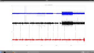
Since my last post I have been investigating training features that can be derived from my Currency Strength indicator as input for machine learning algorithms and during this work it was obvious that there are instances in the raw data that are Black Swan outliers. This can be seen in the chart below as pronounced spikes.
The chart itself is a plot of log returns of various forex crosses and Gold and Silver log returns, concatenated into one long vector. The black is the actual return of the underlying, the blue is the return of the base currency and the red is the cross currency, both of these being calculated from indices formed from the currency strength indicator.

By looking at the dates these spikes occur and then checking online I have flagged four historical "Black swan" events that occured within the time frame the data covers, which are listed in chronological order below:
  1. Precious metals price collapse in mid April 2013
  2. Swiss Franc coming off its peg to the Euro in January 2015
  3. Fears over the Hong Kong dollar and Renminbi currency peg in January 2016
  4. Brexit black Friday
The next series of charts shows the progressive reduction in the number of spikes as the data around the above events is deleted from those crosses etc. that were affected.


It can be seen that the final chart shows much more homogeneous data within each concatenated series, which should have benefits when said data is used as machine learning input. Also, the data that has been deleted will provide a useful, extreme test set to stress test any finished model. More in due course.

Tuesday 12 June 2018

candle.m Function Released

I have just noticed that my previously accepted candlestick plot function now appears to have been released, release date 14 December 2017, as part of the Octave financial package. The function reference is at https://octave.sourceforge.io/financial/function/candle.html 

Thursday 7 June 2018

Update on Improved Currency Strength Indicator

Following on from my previous post I have now slightly changed the logic and coding behind the idea, which can be seen in the code snippet below
%  aud_cad
mse_vector(1) = log( ( current_data(1,1) * ( aud_x / cad_x ) ) / current_data(2,1) )^2 ;
%  xau_aud
mse_vector(46) = log( ( current_data(1,46) * ( gold_x / aud_x ) ) / current_data(2,46) )^2 ;
%  xau_cad
mse_vector(47) = log( ( current_data(1,47) * ( gold_x / cad_x ) ) / current_data(2,47) )^2 ;
Essentially the change simultaneously optimises, using Octave's fminunc function, for both the gold_x and all currency_x geometric multipliers together rather than just optimising for gold and then analytically deriving the currency multipliers. The rationale for this change is shown in the chart below,
which shows the optimisation errors for the "old" way of doing things, in black, and the revised way in blue. Note that this is a log scale, so the errors for the revised way are orders of magnitude smaller, implying a better model fit to the data.

This next chart shows the difference between the two methods of calculating a gold index ( black is old, blue is new ),
this one shows the calculated USD index
and this one the GBP index in blue, USD in green and the forex pair cross rate in black
The idea(s) I am going to look at next is using these various calculated indices as inputs to algorithms/trading decisions.

Monday 28 May 2018

An Improved Currency Strength Indicator plus Gold and Silver Indices?

In the past I have blogged about creating a currency strength indicator ( e.g. here, here and here ) and this post talks about a new twist on this idea.

The motivation for this came about from looking at chart plots such as this,
which shows Gold prices in the first row, Silver in the second and a selection of forex cross rates in the third and final row. The charts are on a daily time scale and show prices since the beginning of 2018 up to and including 25th May, data from Oanda.

If one looks at the price of gold and asks oneself if the price is moving up or down, the answer will depend on which gold price currency denomination chart one looks at. In the latter part of the charts ( from about time ix 70 onwards ) the gold price goes up in pounds Sterling and Euro and down in US dollars. Obviously, by looking at the relevant exchange rates in the third row, a large part of this gold price movement is due to changes in the strength of the underlying currencies. Therefore, the problem to be addressed is that movements in the price of gold are confounded with movements in the price of the currencies, and it would be ideal if the gold price movement could be separated out from the currency movements, which would then allow for the currency strengths to also be determined.

One approach I have been toying with is to postulate a simple, geometric change model whereby the price of gold is multiplied by a constant, let's call it x_g, for example x_g = 1.01 represents a 1% increase in the "intrinsic" value of gold, and then adjust the obtained value of this multiplication to take in to account the change in the value of the currency. The code box below expresses this idea, in somewhat clunky Octave code.
% xau_gbp using gbp_usd
new_val_gold_in_old_currency_value = current_data(1,1) * x_g ;
new_val_gold_in_new_currency_value = new_val_gold_in_old_currency_value * exp( -log( current_data(2,6) / current_data(1,6) ) ) ;
mse_vector(1) = log( current_data(2,1) / new_val_gold_in_new_currency_value )^2 ; 

% xau_usd using gbp_usd
new_val_gold_in_old_currency_value = current_data(1,2) * x_g ;
new_val_gold_in_new_currency_value = new_val_gold_in_old_currency_value * exp( log( current_data(2,6) / current_data(1,6) ) ) ;
mse_vector(2) = log( current_data(2,2) / new_val_gold_in_new_currency_value )^2 ; 
For this snippet, current_data is a 2-dimensional vector containing yesterday's and today's gold prices in GBP and USD, plus yesterday's and today's GBP_USD exchange rates.

The above would be repeated for all gold price currency denominations and the relevant forex pairs and be part of a function, for x_g, which is to be minimised by the Octave fminunc function. Observant readers might note that the error to be minimised is the square of the log of the accuracy ratio. Interested readers are referred to the paper A Better Measure of Relative Prediction Accuracy for Model Selection and Model Estimation for an explanation of this and why it is a suitable error metric for a geometric model.

The chart below is a repeat of the one above, with the addition of a gold index, a silver index and currency strengths indices calculated from a preliminary subset of all gold price currency denominations using the above methodology.
In the first two rows, the blue lines are the calculated gold and silver indices, all normalised to start at the first price at the far left of each respective currency denomination. The silver index was calculated using the relationship between the gold x_g value and the xau xag ratio. Readers will see that these indices are similarly invariant to the currency in which they are expressed ( the geometric bar to bar changes in the indices are identical ) but each is highly correlated to its underlying currency. They could be calculated from an arbitrary index starting point, such as 100, and therefore can be considered to be an index of the changes in the intrinsic value of gold.

When it comes to currency strengths most indicators I have come across are variations of a single theme, namely: averages of all the changes for a given set of forex pairs, whether these changes be expressed as logs, percentages, values or whatever. Now that we have an absolute, intrinsic value gold index, it is a simple matter to parse out the change in the currency from the change in the gold price in this currency.

The third row of the second chart above shows these currency strengths for the two base currencies plotted - GBP and EUR - again normalised to the first charted price on the left. Although in this chart only observable for the Euro, it can be seen that the index again is invariant, similar to gold and silver above. Perhaps more interestingly, the red line is a cumulative product of the ratio of base currency index change to the term currency index change, normalised as described above. It can be seen that the red line almost exactly overwrites the underlying black line, which is the actual cross rate plot. This red line is plotted as a sanity check and it is gratifying to see such an accurate overwrite.

I think this idea shows great promise and for the nearest future I shall be working to extend it beyond the preliminary data set used above. More in due course.

Friday 2 March 2018

Hidden Markov Modelling of Synthetic Periodic Time Series Data

I am currently working on a method of predicting/projecting cyclic price action, based upon John Ehlers' sinewave indicator code, and to test it I am using Octave's implementation of a Hidden Markov model in the Octave statistics package hosted at Sourceforge.

Basically I measure the dominant cycle period ( using either the above linked sinewave indicator code or autocorrelation periodogram code ) and use the vector of measured dominant cycle periods as input to the hmmestimate function. Using the output from this, the hmmgenerate function is then used to generate a new period vector, these periods are converted to a slowly, periodically varying sine wave, and additive white Gaussian noise is added to the signal to produce a final signal upon which Monte Carlo testing of my proposed indicator can be conducted. A typical plot of the varying, dominant cycle periods looks like
whilst the noisy sine wave signal derived from this looks like this.
The relevant Octave code for all this is shown in the two code boxes below
clear all ;
pkg load statistics ;

% load all datafile names from Oanda
cd /home/dekalog/Documents/octave/oanda_data/daily ;
oanda_files_d = glob( "*_ohlc_daily" ) ; % cell with filenames matching *_ohlc_daily, e.g. eur_usd_ohlc_daily

all_transprobest = zeros( 75 , 75 ) ;

for ii = 1 : 124

filename = oanda_files_d{ ii } ; 
current_data_d = load( "-binary" , filename ) ;
data = getfield( current_data_d , filename ) ; 
midprice = ( data( : , 3 ) .+ data( : , 4 ) ) ./ 2 ;
period = autocorrelation_periodogram_2_5( midprice ) ;
period(1:49) = [] ;
min_val = min( period ) ; max_val = max( period ) ;
hmm_periods = period .- ( min_val - 1 ) ; hmm_states = hmm_periods ;

[ transprobest , outprobest ] = hmmestimate( hmm_periods , hmm_states ) ;
all_transprobest( min_val : max_val , min_val : max_val ) = all_transprobest( min_val : max_val , min_val : max_val ) .+ transprobest ;

endfor

all_transprobest = all_transprobest ./ 124 ;
[ i , j ] = find( all_transprobest ) ;

if ( min(i) == min(j) && max(i) == max(j) )
transprobest = all_transprobest( min(i):max(i) , min(j):max(j) ) ;
outprobest = eye( size(transprobest,1) ) ;
hmm_min_period_add = min(i) - 1 ;
endif

cd /home/dekalog/Documents/octave/period/hmm_period ;
save all_hmm_periods_daily transprobest outprobest hmm_min_period_add ;
and
clear all ;
pkg load statistics ;
cd /home/dekalog/Documents/octave/snr ;
load all_snr ;
cd /home/dekalog/Documents/octave/period/hmm_period ;
load all_hmm_periods_daily ;

[ gen_period , gen_states ] = hmmgenerate( 2500 , transprobest , outprobest ) ;
gen_period = gen_period .+ hmm_min_period_add ;
gen_sine = sind( cumsum( 360 ./ gen_period ) ) ;
noise_val = mean( [ all_snr(:,1) ; all_snr(:,2) ] ) ;
noisy_sine = awgn( gen_sine , noise_val ) ;
[s,s1,s2,s3] = sinewave_indicator( noisy_sine ) ; s2(1:50) = s1(1:50) ;

figure(1) ; plot( gen_period , 'k' , 'linewidth' , 2 ) ; 
figure(2) ; plot( gen_sine , 'k' , 'linewidth' , 2 , noisy_sine , 'b' , 'linewidth' , 2 , s , 'r' , 'linewidth' , 2 , ...
s1 , 'g' , 'linewidth' , 2 , s2 , 'm' , 'linewidth' , 2 ) ;
legend( "Gen Sine" , "Noisy Sine" , "Sine Ind" , "Sine Ind lead1" , "Sine Ind Lead2" ) ;
I hope readers find this useful if they need to generate synthetic, cyclic data for their own development/testing purposes too.