Showing posts with label Cycle Period. Show all posts

Tuesday, 9 April 2024

A "New" Use for Kalman Filter on Price Time Series?

During the course of writing this blog I have visited the idea of using Kalman filters several times, most recently in this February 2023 post. My motivation in these previous posts could best be described as trying to smooth price data with as little lag as possible, i.e. create a zero-lag indicator. In doing so, the model most often used for the Kalman filter was a physical motion model with position, velocity and acceleration components. Whilst these "worked" in the sense of smoothing the underlying data, it is not necessarily a good model to use on financial data because, obviously, financial data is not a physical system and so I thought I would apply the Kalman filter to something that is ubiquitously used on financial data - the Exponential moving average.

Below is an Octave function to calculate a "Kalman_ema" where the prediction part of the filter is just a linear extrapolation of an exponential moving average and then this extrapolated value is used to calculate the projected price, with the measurement being the real price and its ema value.

## Copyright (C) 2024 dekalog
##
## This program is free software: you can redistribute it and/or modify
## it under the terms of the GNU General Public License as published by
## the Free Software Foundation, either version 3 of the License, or
## (at your option) any later version.
##
## This program is distributed in the hope that it will be useful,
## but WITHOUT ANY WARRANTY; without even the implied warranty of
## MERCHANTABILITY or FITNESS FOR A PARTICULAR PURPOSE.  See the
## GNU General Public License for more details.
##
## You should have received a copy of the GNU General Public License
## along with this program.  If not, see .

## -*- texinfo -*-
## @deftypefn {} {@var{retval} =} kalman_ema (@var{price}, @var{lookback})
##
## @seealso{}
## @end deftypefn

## Author: dekalog 
## Created: 2024-04-08

function [ filter_out , P_out ] = kalman_ema ( price , lookback )

## check price is row vector
if ( size( price , 1 ) > 1 && size( price , 2 ) == 1 )
 price = price' ;
endif

P_out = zeros( numel( price ) , 2 ) ;

ema_price = ema( price , lookback )' ;
alpha = 2 / ( lookback + 1 ) ;

## initial covariance matrix
P = eye( 3 ) ;

## transistion matrix
A = [ 0 , ( 1 + alpha ) / alpha , -( 1 / alpha ) ; ...
       0 , 2 , -1 ; ...
       0 , 1 , 0 ] ;

## initial Q
Q = eye( 3 ) ;

## measurement vector
Y = [ price ; ...
       ema_price ; ...
       shift( ema_price , 1 ) ] ;
Y( 3 , 1 ) = Y( 2 , 1 ) ;

## measurement matrix
H = eye( 3 ) ;

## measurement noise covariance
R = eye( 3 ) ;

## container for Kalman filter output
filter_out = zeros( size( Y ) ) ;
errors = ones( 3 , 1 ) ;

for ii = 2 : size( Y , 2 )

  X = A * filter_out( : , ii - 1 ) ;
  P = A * P * A' + Q ;

  errors = alpha .* abs( X - Y( : , ii ) ) + ( 1 - alpha ) .* errors ;

  IM = H * X ; ## Mean of predictive distribution
  IS = ( R + H * P * H' ) ; ## Covariance of predictive mean
  K = P * H' / IS ; ## Computed Kalman gain
  X = X + K * ( Y( : , ii ) - IM ) ; ## Updated state mean
  P = P - K * IS * K' ; ## Updated state covariance

  filter_out( : , ii ) = X ;
  P_out( ii , 1 ) = P( 1 , 1 ) ;
  P_out( ii , 2 ) = P( 2 , 2 ) ;

  ## update Q and R
  Q( 1 , 1 ) = errors( 1 ) ; Q( 2 , 2 ) = errors( 2 ) ; Q( 3 , 3 ) = errors( 3 ) ;
  R = Q ;

endfor

filter_out = filter_out' ;

endfunction
Using this for smoothing either the price or the ema has no utility, but a by-product of the filter is the Covariance matrix from which it is possible to plot bands around the price series. The following chart shows the bands for various ema alpha values corresponding to various Fibonacci sequence length look backs for the ema alpha value.  
This next chart, for purposes of clarity, shows the "Golden Cross" lengths of 50 and 200
and this final chart shows an adaptive look back length which is a function of the instantaneous measured period (see here or here) of the underlying data.

Despite the wide range of the input look back lengths for the ema, it can be seen that the covariance bands around price are broadly similar. I can think of many uses for such a data driven but basically parameter insensitive measure of price variance, e.g. entry/exit levels, stop levels, position sizing etc.

More in due course.


Tuesday, 28 February 2023

Kalman Filter and Sensor Fusion.

In the Spring of 2012 and again in the Spring of 2019 I posted a series of posts about the Kalman Filter, which readers can access via the blog archive on the right. In both cases I eventually gave up those particular lines of investigation because of disappointing results. This post is the first in a new series about using the Kalman Filter for sensor fusion, which I had known of before, but due to the paucity of clear information about this online I had never really investigated. However, my recent discovery of this Github and its associated online tutorial has inspired me to a third attempt at using Kalman Filters. What I am going to attempt to do is use the idea of sensor fusion to fuse the output of several functions I have coded in the past, which each extract the dominant cycle from a time series, to hopefully obtain a better representation of the "true underlying cycle."

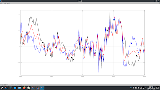
The first step in this process is to determine the measurement noise covariance or, in Kalman Filter terms, the "R" covariance matrix. To do this, I have used the average of two of the outputs from the above mentioned functions to create a new cycle and similarly used two extracted trends (price minus these cycles) averaged to get a new trend. The new cycle and new trend are simply added to each other to create a new price series which is almost identical to the original price series. The screenshot below shows a typical cycle extract,

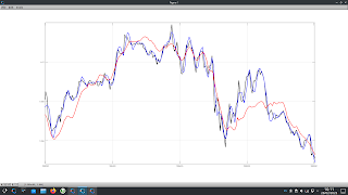
where the red cycle is the average of the other two extracted cycles, and this following screenshot shows the new trend in red plus the new price alongside the old price (blue and black respectively).
Having created a time series thus with known trend and cycle, it is a simple matter to run my cycle extractor functions on this new price, compare the outputs with the known cyclic component of price and calculate the variance of the errors to get the R covariance matrices for 14 different currency crosses.

More in due course.
 

Friday, 29 November 2019

RVFL Network Results

Having let the tests outlined in my previous post run, I can say that the results are inconclusive as the optimised number of neurons in the hidden layer turns out to be one, the minimum possible to even have a hidden layer. This leads me to believe that the raw features, the ideal cyclic tau embedding, are sufficient in and of themselves for the purpose I have in mind.

To that end, I have indulged in a bit of feature engineering and written the following Octave function,
## Copyright (C) 2019 dekalog
## 
## This program is free software: you can redistribute it and/or modify it
## under the terms of the GNU General Public License as published by
## the Free Software Foundation, either version 3 of the License, or
## (at your option) any later version.
## 
## This program is distributed in the hope that it will be useful, but
## WITHOUT ANY WARRANTY; without even the implied warranty of
## MERCHANTABILITY or FITNESS FOR A PARTICULAR PURPOSE.  See the
## GNU General Public License for more details.
## 
## You should have received a copy of the GNU General Public License
## along with this program.  If not, see
## www.gnu.org.

## -*- texinfo -*- 
## @deftypefn {} {@var{emb1}, @var{emb2} =} cyclic_embedding (@var{price}, @var{period})
##
## Inputs are a price vector and a period vector.
##
## The function normalises the price between -1 and +1 over an adaptive period lookback.
##
## The outputs are two matrices of 3 columns each - the first column is normalised price
## and the second and third are delay embeddings of Tau and 2 x Tau, Tau being equal to
## one quarter of the adaptive period vector, the theoretical ideal Tau for sinusoidal
## waveforms.
##
## The first output matrix, EMB1, normalises the Tau and 2 x Tau columns according to the
## most recent max high/min low; EMB2 Tau and 2 x Tau are normalised according to the 
## max high/min low in force at the delay embedding time.
##
## @seealso{}
## @end deftypefn

## Author: dekalog 
## Created: 2019-09-18

function [ emb1 , emb2 , prob_matrix ] = cyclic_embedding( price , period )
  
price_smooth = price ;
emb1 = repmat( price , 1 , 3 ) ;
emb2 = emb1 ;
coeffs = generalised_sgolay_filter_coeffs( 5 , 2 , 0 ) ; coeffs = coeffs' ;

## initialising loop
price_smooth( 1 : 3 ) = coeffs( 1 : 3 , : ) * price( 1 : 5 ) ;  
for ii = 4 : 48 
  price_smooth( ii ) = coeffs( 3 , : ) * price( ii - 2 : ii + 2 ) ;
endfor
price_smooth( 49 : 50 ) = coeffs( 4 : 5 , : ) * price( 46 : 50 ) ;
## end initialising loop 

coeffs( 1 : 2 , : ) = [] ;

for ii = 51 : size( price , 1 )

  price_smooth( ii - 2 : ii ) = coeffs * price( ii - 4 : ii ) ;
  max_r = max( price_smooth( ii - period( ii ) : ii ) ) ;
  min_r = min( price_smooth( ii - period( ii ) : ii ) ) ;
  
  ## period is exactly divisable by 4 ( and 2 ), e.g. 8 12 16 20 24 28 32 36 40 44 48 etc?
  if ( rem( period( ii ) , 4 ) == 0 ) 
    
  emb1( ii , 1 ) = 2 * ( ( price_smooth( ii ) - min_r ) / ( max_r - min_r ) - 0.5 ) ;
  emb1( ii , 2 ) = 2 * ( ( price_smooth( ii - round( period( ii ) / 4 ) ) - min_r ) / ( max_r - min_r ) - 0.5 ) ;
  emb1( ii , 3 ) = 2 * ( ( price_smooth( ii - round( period( ii ) / 2 ) ) - min_r ) / ( max_r - min_r ) - 0.5 ) ;
  emb2( ii , 1 ) = emb1( ii , 1 ) ;
  emb2( ii , 2 ) = emb2( ii - round( period( ii ) / 4 ) , 1 ) ;
  emb2( ii , 3 ) = emb2( ii - round( period( ii ) / 2 ) , 1 ) ;
  
  ## periods 10 14 18 22 26 30 34 38 42 46 50
  elseif ( rem( period( ii ) , 2 ) == 0 && rem( period( ii ) , 4 ) == 2 )

  emb1( ii , 1 ) = 2 * ( ( price_smooth( ii ) - min_r ) / ( max_r - min_r ) - 0.5 ) ;
  emb1( ii , 2 ) = 2 * ( ( ( 0.5*price_smooth( ii - round( period( ii ) / 4 ) ) + 0.5*price_smooth( ii - round( period( ii ) / 4 ) + 1 ) ) - min_r )...
                       / ( max_r - min_r ) - 0.5 ) ;
  emb1( ii , 3 ) = 2 * ( ( price_smooth( ii - round( period( ii ) / 2 ) ) - min_r ) / ( max_r - min_r ) - 0.5 ) ;
  emb2( ii , 1 ) = emb1( ii , 1 ) ;
  emb2( ii , 2 ) = 0.5*emb2( ii - round( period( ii ) / 4 ) , 1 ) + 0.5*emb2( ii - round( period( ii ) / 4 ) + 1 , 1 ) ;
  emb2( ii , 3 ) = emb2( ii - round( period( ii ) / 2 ) , 1 ) ;

  ## periods 9 13 17 21 25 29 33 37 41 45 49
  elseif ( rem( period( ii ) , 2 ) == 1 && rem( period( ii ) , 4 ) == 1 )

  emb1( ii , 1 ) = 2 * ( ( price_smooth( ii ) - min_r ) / ( max_r - min_r ) - 0.5 ) ;
  emb1( ii , 2 ) = 2 * ( ( ( 0.75*price_smooth( ii - round( period( ii ) / 4 ) ) + 0.25*price_smooth( ii - round( period( ii ) / 4 ) - 1 ) ) - min_r )...
                       / ( max_r - min_r ) - 0.5 ) ;
  emb1( ii , 3 ) = 2 * ( ( ( 0.5*price_smooth( ii - round( period( ii ) / 2 ) ) + 0.5*price_smooth( ii - round( period( ii ) / 2 ) + 1 ) ) - min_r )...
                       / ( max_r - min_r ) - 0.5 ) ;
  emb2( ii , 1 ) = emb1( ii , 1 ) ;
  emb2( ii , 2 ) = 0.75*emb2( ii - round( period( ii ) / 4 ) , 1 ) + 0.25*emb2( ii - round( period( ii ) / 4 ) - 1 , 1 ) ;
  emb2( ii , 3 ) = 0.5*emb2( ii - round( period( ii ) / 2 ) , 1 ) + 0.5*emb2( ii - round( period( ii ) / 2 ) + 1 , 1 ) ;
  
  ## periods 11 15 19 23 27 31 35 39 43 47
  elseif ( rem( period( ii ) , 2 ) == 1 && rem( period( ii ) , 4 ) == 3 )

  emb1( ii , 1 ) = 2 * ( ( price_smooth( ii ) - min_r ) / ( max_r - min_r ) - 0.5 ) ;
  emb1( ii , 2 ) = 2 * ( ( ( 0.75*price_smooth( ii - round( period( ii ) / 4 ) ) + 0.25*price_smooth( ii - round( period( ii ) / 4 ) + 1 ) ) - min_r )...
                       / ( max_r - min_r ) - 0.5 ) ;
  emb1( ii , 3 ) = 2 * ( ( ( 0.5*price_smooth( ii - round( period( ii ) / 2 ) ) + 0.5*price_smooth( ii - round( period( ii ) / 2 ) + 1 ) ) - min_r )...
                       / ( max_r - min_r ) - 0.5 ) ;
  emb2( ii , 1 ) = emb1( ii , 1 ) ;
  emb2( ii , 2 ) = 0.75*emb2( ii - round( period( ii ) / 4 ) , 1 ) + 0.25*emb2( ii - round( period( ii ) / 4 ) + 1 , 1 ) ;
  emb2( ii , 3 ) = 0.5*emb2( ii - round( period( ii ) / 2 ) , 1 ) + 0.5*emb2( ii - round( period( ii ) / 2 ) + 1 , 1 ) ;
  
  endif
  
endfor ## end of embedding features creation

feature_peak = emb2 * [ 1 0 ; -1 1 ; 0 -1 ] * [ 1 ; 1 ] ;
feature_trough = zeros( size( feature_peak ) ) ;
ix = find( feature_peak < 0 ) ; 
feature_trough( ix ) = abs( feature_peak( ix ) ) ;
feature_peak( feature_peak <= 0 ) = 0 ;

## https://stats.stackexchange.com/questions/132652/how-to-determine-which-distribution-fits-my-data-best
## Weibull distribution with shape = 219.68 and scale = 1.94 for turn +/- 1 bar
## Weibull distribution with shape = 85.88 and scale = 1.84 for turn +/- 2 bar
## This comes from bayesian testing of cutoff value of feature_peak/feature_trough for highs/lows +/- 1 bar.
## The function used to get these values is "bayes_train_cyclic_turn_prob_of_embedding.m" which calls
## "bayes_optim_of_cyclic_embedding_conv_function" in /home/dekalog/Documents/octave/turning_points
scale = 1.84 ; shape = 85.88 ;
prob_matrix = zeros( size( feature_peak , 1 ) , 3 ) ;
prob_matrix( : , 1 ) = wblcdf( feature_peak , scale , shape ) ;
prob_matrix( : , 2 ) = wblcdf( feature_trough , scale , shape ) ;
prob_matrix( : , 3 ) = 1 .- sum( prob_matrix( : , 1 : 2 ) , 2 ) ;

endfunction
which again is a work in progress.

This takes as input a price and a period vector and outputs features as per the plots in the above linked ideal cyclic tau post plus a matrix of probabilities for price action being at a cyclic high/low. This matrix is the result of Monte Carlo Bayesian Optimisation over ideal sine wave prices to get a cutoff value for the derived feature in the above function. The probability distribution used for this probability matrix is the Weibull distribution, which has been determined by following the routine outlined in this "how to determine which distribution fits my data best" forum post and using the R statistical software platform.

The hard coded values for the cutoff in the above code are from the results of optimisation on pure sine waves. As I write this post there are optimisation routines running on sine waves with 20 db noise added.

More in due course.

Tuesday, 1 October 2019

Ideal Cyclic Tau Embedding as Times Series Features

Continuing on from my Ideal Tau for Time Series Embedding post, I have now written an Octave function based on these ideas to produce features for time series modelling. The function outputs are two slightly different versions of features, examples of which are shown in the following two plots, which show up and down trends in black, following a sinusoidal sideways market partially visible to the left:
and

The function outputs are normalised price and price delayed by a quarter and a half of the cycle period (in this case 20.) The trend slopes have been chosen to exemplify the difference in the features between up and down trends. The function outputs are identical for the unseen cyclic prices to the left.

When the sets of function outputs are plotted as 3D phase space plots typical results are
with the green, blue and red phase trajectories corresponding to the cyclic, up trending and down trending portions of the above synthetic price series. The markers in this plot correspond to points in the phase trajectories at which turns in the underlying price series occur. The following plot is the above plot rotated in phase space such that the green cyclic price phase trajectory is horizontally orientated.
It is clearer in this second phase space plot that there is a qualitative difference in the phase space trajectories of the different, underlying market types.

As a final check of feature relevance I used the Boruta R package, with the above turning point markers as classification targets (a turning point vs. not a turning point,) to assess the utility of this approach in general. These tests were conducted on real price series and also on indices created by my currency strength methodology. In all such Boruta tests the features are deemed "relevant" up to a delay of five bars on daily data (I ceased the tests at the five bar mark because it was becoming tedious to carry on.)

In summary, therefore, it can be concluded that features derived using Taken's theorem are useful on financial time series provided that:
  1. the underlying time series are normalised (detrended) and,
  2. the embedding delay (Tau) is set to the theoretical optimum of a quarter (and multiples thereof) of the measured cyclic period of the time series.

Thursday, 5 September 2019

Preliminary Test Results of Time Series Embedding

Following on from my post yesterday, this post presents some preliminary results from the test I was running while writing yesterday's post. However, before I get to these results I would like to talk a bit about the hypothesis being tested.

I had an inkling that the dominant cycle period might having some bearing on tau, the time delay for the time series embedding implied by Taken's theorem, so I set up the test (described below) and after writing the post yesterday, and while the test was still running, I did some online research to see if there is any theoretical justification available.

One of the papers I found online is A Novel Method for Topological Embedding of Time-Series Data. From the abstract

"...we propose a novel method for embedding one-dimensional, periodic time-series data into higher-dimensional topological spaces to support robust recovery of signal features via topological data analysis under noisy sampling conditions...To provide evidence for the viability of this method, we analyze the simple case of sinusoidal data..."

One of the conclusions drawn is that for sinusoidal data the ideal embedding length is a quarter of the cycle period, i.e. Π/2.

Another paper I found was Topological time-series analysis with delay-variant embedding. This paper investigates "delay-variant embedding," essentially making the embedding length tau variable. From the concluding remarks

"We have demonstrated that the topological features that are constructed using delay-variant embedding can capture the topological variation in a time series when the time-delay value changes... These results indicate that the topological features that are deduced with delay-variant embedding can be used to reveal the representative features of the original time series."

My inkling was that tau should be adaptive to the measured dominant cycle, and both the above linked papers do provide some justification. Anyway, on to the test.

Reusing the code from my earlier post here I created synthetic price series with known but variable dominant cycle periods and based on real price trends, which results in synthetic series that are highly correlated with real price series but with underlying characteristics being exactly known. I then used my version of mdembedding code to calculate tau for numerous Monte Carlo replications of time series of prices based on a range of real forex pairs prices, gold and silver prices and different indices created by my currency strength indicator methodology. I then created a ratio of tau/average_measured_period measured as a global value across the whole of each individual time series replication as the test statistic, with the period being measured by an autocorrelation periodogram function: a ratio value of 0.5, for example, meaning that the tau for that time series is half the average period over the whole series.

Below is a plot of the histogram of these ratios:
which shows the ratios being centred approximately around 0.4 but with a long right tail. The following histogram is of the means of the bootstrap with replacement of the above distribution,
which is centred around a mean value of 0.436. Using this bootstrapped mean ratio of tau/period implies, for example, that the ideal tau for an average period of 20 is 8.72, which when rounded up to 9, is almost twice the theoretical ideal of a 5 day tau for 20 day cyclic period prices.

Personally I think this is an encouraging set of preliminary test results, with some caveats. More in due course.

Friday, 2 March 2018

Hidden Markov Modelling of Synthetic Periodic Time Series Data

I am currently working on a method of predicting/projecting cyclic price action, based upon John Ehlers' sinewave indicator code, and to test it I am using Octave's implementation of a Hidden Markov model in the Octave statistics package hosted at Sourceforge.

Basically I measure the dominant cycle period ( using either the above linked sinewave indicator code or autocorrelation periodogram code ) and use the vector of measured dominant cycle periods as input to the hmmestimate function. Using the output from this, the hmmgenerate function is then used to generate a new period vector, these periods are converted to a slowly, periodically varying sine wave, and additive white Gaussian noise is added to the signal to produce a final signal upon which Monte Carlo testing of my proposed indicator can be conducted. A typical plot of the varying, dominant cycle periods looks like
whilst the noisy sine wave signal derived from this looks like this.
The relevant Octave code for all this is shown in the two code boxes below
clear all ;
pkg load statistics ;

% load all datafile names from Oanda
cd /home/dekalog/Documents/octave/oanda_data/daily ;
oanda_files_d = glob( "*_ohlc_daily" ) ; % cell with filenames matching *_ohlc_daily, e.g. eur_usd_ohlc_daily

all_transprobest = zeros( 75 , 75 ) ;

for ii = 1 : 124

filename = oanda_files_d{ ii } ; 
current_data_d = load( "-binary" , filename ) ;
data = getfield( current_data_d , filename ) ; 
midprice = ( data( : , 3 ) .+ data( : , 4 ) ) ./ 2 ;
period = autocorrelation_periodogram_2_5( midprice ) ;
period(1:49) = [] ;
min_val = min( period ) ; max_val = max( period ) ;
hmm_periods = period .- ( min_val - 1 ) ; hmm_states = hmm_periods ;

[ transprobest , outprobest ] = hmmestimate( hmm_periods , hmm_states ) ;
all_transprobest( min_val : max_val , min_val : max_val ) = all_transprobest( min_val : max_val , min_val : max_val ) .+ transprobest ;

endfor

all_transprobest = all_transprobest ./ 124 ;
[ i , j ] = find( all_transprobest ) ;

if ( min(i) == min(j) && max(i) == max(j) )
transprobest = all_transprobest( min(i):max(i) , min(j):max(j) ) ;
outprobest = eye( size(transprobest,1) ) ;
hmm_min_period_add = min(i) - 1 ;
endif

cd /home/dekalog/Documents/octave/period/hmm_period ;
save all_hmm_periods_daily transprobest outprobest hmm_min_period_add ;
and
clear all ;
pkg load statistics ;
cd /home/dekalog/Documents/octave/snr ;
load all_snr ;
cd /home/dekalog/Documents/octave/period/hmm_period ;
load all_hmm_periods_daily ;

[ gen_period , gen_states ] = hmmgenerate( 2500 , transprobest , outprobest ) ;
gen_period = gen_period .+ hmm_min_period_add ;
gen_sine = sind( cumsum( 360 ./ gen_period ) ) ;
noise_val = mean( [ all_snr(:,1) ; all_snr(:,2) ] ) ;
noisy_sine = awgn( gen_sine , noise_val ) ;
[s,s1,s2,s3] = sinewave_indicator( noisy_sine ) ; s2(1:50) = s1(1:50) ;

figure(1) ; plot( gen_period , 'k' , 'linewidth' , 2 ) ; 
figure(2) ; plot( gen_sine , 'k' , 'linewidth' , 2 , noisy_sine , 'b' , 'linewidth' , 2 , s , 'r' , 'linewidth' , 2 , ...
s1 , 'g' , 'linewidth' , 2 , s2 , 'm' , 'linewidth' , 2 ) ;
legend( "Gen Sine" , "Noisy Sine" , "Sine Ind" , "Sine Ind lead1" , "Sine Ind Lead2" ) ;
I hope readers find this useful if they need to generate synthetic, cyclic data for their own development/testing purposes too.

Thursday, 27 October 2016

Currency Strength Indicator

Over the last few weeks I have been looking into creating a currency strength indicator as input to a Nonlinear autoregressive exogenous model. This has involved a fair bit of online research and I have to say that compared to other technical analysis indicators there seems to be a paucity of pages devoted to the methodology of creating such an indicator. Apart from the above linked Wikipedia page I was only really able to find some discussion threads on some forex forums, mostly devoted to the Metatrader platform, and a few of the more enlightening threads are here, here and here. Another website I found, although not exactly what I was looking for, is marketsmadeclear.com and in particular their Currency Strength Matrix.

In the end I decided to create my own relative currency strength indicator, based on the RSI, by making the length of the indicator adaptive to the measured dominant cycle. The optimal theoretical length for the RSI is half the cycle period, and the price series are smoothed in a [ 1 2 2 1 ] FIR filter prior to the RSI calculations. I used the code in my earlier post to calculate the dominant cycle period, the reason being that since I wrote that post I have watched/listened to a podcast in which John Ehlers recommended using this calculation method for dominant cycle measurement.

The screenshots below are of the currency strength indicator applied to approx. 200 daily bars of the EURUSD forex pair; first the price chart,
next, the indicator,
and finally an oscillator derived from the two separate currency strength lines.
I think the utility of this indicator is quite obvious from these simple charts. Crossovers of the strength lines ( or equivalently, zero line crossings of the oscillator ) clearly indicate major directional changes, and additionally changes in the slope of the oscillator provide an early warning of impending price direction changes.

I will now start to test this indicator and write about these tests and results in due course.

Monday, 16 May 2016

Giving Up on Recursive Sine Formula for Period Calculation

I have spent the last few weeks trying to get my recursive sine wave formula for period calculations to work, but try as I might I can only get it to do so under ideal theoretical conditions. Once any significant noise, trend or combination thereof is introduced the calculations explode and give meaningless results. In light of this, I am no longer going to continue this work.

Apart from the above work I have also been doing my usual online research and have come across John Ehler's autocorrelation periodogram for period measurement, and below is my Octave C++ .oct implementation of it.
DEFUN_DLD ( autocorrelation_periodogram, args, nargout,
"-*- texinfo -*-\n\
@deftypefn {Function File} {} autocorrelation_periodogram (@var{input_vector})\n\
This function takes an input vector ( price ) and outputs the dominant cycle period,\n\
calculated from the autocorrelation periodogram spectrum.\n\
@end deftypefn" )

{
octave_value_list retval_list ;
int nargin = args.length () ;

// check the input arguments
if ( nargin != 1 ) // there must be a price vector only
   {
   error ("Invalid arguments. Input is a price vector only.") ;
   return retval_list ;
   }

if ( args(0).length () < 4 )
   {
   error ("Invalid argument length. Input is a price vector of length >= 4.") ;
   return retval_list ;
   }

if ( error_state )
   {
   error ("Invalid argument. Input is a price vector of length >= 4.") ;
   return retval_list ;
   }
// end of input checking 

ColumnVector input = args(0).column_vector_value () ;
ColumnVector hp = args(0).column_vector_value () ; hp.fill( 0.0 ) ;
ColumnVector smooth = args(0).column_vector_value () ; smooth.fill( 0.0 ) ;
ColumnVector corr ( 49 ) ; corr.fill( 0.0 ) ;
ColumnVector cosine_part ( 49 ) ; cosine_part.fill( 0.0 ) ;
ColumnVector sine_part ( 49 ) ; sine_part.fill( 0.0 ) ;
ColumnVector sq_sum ( 49 ) ; sq_sum.fill( 0.0 ) ;
ColumnVector R1 ( 49 ) ; R1.fill( 0.0 ) ;
ColumnVector R2 ( 49 ) ; R2.fill( 0.0 ) ;  
ColumnVector pwr ( 49 ) ; pwr.fill( 0.0 ) ;
ColumnVector dominant_cycle = args(0).column_vector_value () ; dominant_cycle.fill( 0.0 ) ;  
   
double avglength = 3.0 ;
double M ;
double X ; double Y ;   
double Sx ; double Sy ; double Sxx ; double Syy ; double Sxy ;
double denom ;
double max_pwr = 0.0 ;
double Spx ; double Sp ;  

// variables for highpass filter, hard coded for a high cutoff period of 48 bars and low cutoff of 10 bars
double high_cutoff = 48.0 ; double low_cutoff = 10.0 ;  
double alpha_1 = ( cos( 0.707 * 2.0 * PI / high_cutoff ) + sin( 0.707 * 2.0 * PI / high_cutoff ) - 1.0 ) / cos( 0.707 * 2.0 * PI / high_cutoff ) ;   
double beta_1 = ( 1.0 - alpha_1 / 2.0 ) * ( 1.0 - alpha_1 / 2.0 ) ;
double beta_2 = 2.0 * ( 1.0 - alpha_1 ) ;
double beta_3 = ( 1.0 - alpha_1 ) * ( 1.0 - alpha_1 ) ;
 
// variables for super smoother
double a1 = exp( -1.414 * PI / low_cutoff ) ;
double b1 = 2.0 * a1 * cos( 1.414 * PI / low_cutoff ) ;
double c2 = b1 ;
double c3 = -a1 * a1 ;
double c1 = 1.0 - c2 - c3 ;
  
// calculate the automatic gain control factor, K
double K = 0.0 ;
double accSlope = -1.5 ; //acceptableSlope = 1.5 dB
double halfLC = low_cutoff / 2.0 ;
double halfHC = high_cutoff / 2.0 ;
double ratio = pow( 10 , accSlope / 20.0 ) ;
  
 if( halfHC - halfLC > 0.0 )
    {
  K = pow( ratio , 1.0 / ( halfHC - halfLC ) ) ;
    }

// loop to initialise hp and smooth
for ( octave_idx_type ii ( 2 ) ; ii < 49 ; ii++ ) // main loop
    {  
    // highpass filter components whose periods are < 48 bars
    hp(ii) = beta_1 * ( input(ii) - 2.0 * input(ii-1) + input(ii-2) ) + beta_2 * hp(ii-1) - beta_3 * hp(ii-2) ;
    
    // smooth with a super smoother filter
    smooth(ii) = c1 * ( hp(ii) + hp(ii-1) ) / 2.0 + c2 * smooth(ii-1) + c3 * smooth(ii-2) ;
    } // end of initial loop

for ( octave_idx_type ii ( 49 ) ; ii < args(0).length () ; ii++ ) // main loop
    {  
    // highpass filter components whose periods are < 48 bars
    hp(ii) = beta_1 * ( input(ii) - 2.0 * input(ii-1) + input(ii-2) ) + beta_2 * hp(ii-1) - beta_3 * hp(ii-2) ;
    
    // smooth with a super smoother filter
    smooth(ii) = c1 * ( hp(ii) + hp(ii-1) ) / 2.0 + c2 * smooth(ii-1) + c3 * smooth(ii-2) ;
      
      // Pearson correlation for each value of lag
      for ( octave_idx_type lag (0) ; lag <= high_cutoff ; lag++ ) 
          {
          // set the averaging length as M
          M = avglength ;
          if ( avglength == 0) 
             {
              M = double( lag ) ; 
             }
             
          Sx = 0.0 ; Sy = 0.0 ; Sxx = 0.0 ; Syy = 0.0 ; Sxy = 0.0 ;
            
            for ( octave_idx_type count (0) ; count < M - 1 ; count++ )
                {
                 X = smooth(ii-count) ; Y = smooth(ii-(lag+count)) ; 
                 Sx += X ; 
                 Sy += Y ;
                 Sxx += X * X ;
                 Sxy += X * Y ;
                 Syy += Y * Y ;
                }
             
            denom = ( M * Sxx - Sx * Sx ) * ( M * Syy - Sy * Sy ) ;    
            if ( denom > 0.0 )
               {
                corr(lag) = ( M * Sxy - Sx * Sy ) / sqrt( denom ) ;  
               }    
            
          } // end of Pearson correlation loop        
/*
    The DFT is accomplished by correlating the autocorrelation at each value of lag with the cosine and sine of each period of interest. 
    The sum of the squares of each of these values represents the relative power at each period.
*/                  
      for ( octave_idx_type period (low_cutoff) ; period <= high_cutoff ; period++ )
          {
           cosine_part( period ) = 0.0 ; sine_part( period ) = 0.0 ;
            
            for ( octave_idx_type N (3) ; N <= high_cutoff ; N++ )
                {
                 cosine_part( period ) += corr( N ) * cos( 2.0 * PI * double( N ) / double( period ) ) ;  
                 sine_part( period ) += corr( N ) * sin( 2.0 * PI * double( N ) / double( period ) ) ; 
                } // end of N loop
                
            sq_sum( period ) = cosine_part( period ) * cosine_part( period ) + sine_part( period ) * sine_part( period ) ;
                
          } // end of first period loop 
 
      // EMA is used to smooth the power measurement at each period          
      for ( octave_idx_type period (low_cutoff) ; period <= high_cutoff ; period++ )
          {
           R2( period ) = R1( period ) ;
           R1( period ) = 0.2 * sq_sum( period ) * sq_sum( period ) + 0.8 * R2( period ) ; 
          } // end of second period loop
      
    // Find maximum power level for normalisation      
    max_pwr = 0.0 ;      
          
      for ( octave_idx_type period (low_cutoff) ; period <= high_cutoff ; period++ )
          {
           if ( R1( period ) > max_pwr )
              {
                max_pwr = K * R1( period ) ;
              }
          } // end of third period loop
    
    // normalisation of power      
      for ( octave_idx_type period (low_cutoff) ; period <= high_cutoff ; period++ )
          {
           pwr( period ) = R1( period ) / max_pwr ;
          } // end of fourth period loop 
      
    // compute the dominant cycle using the centre of gravity of the spectrum
    Spx = 0.0 ; Sp = 0.0 ;
    
      for ( octave_idx_type period (low_cutoff) ; period <= high_cutoff ; period++ )
          {
           if ( pwr( period ) >= 0.5 )
              {
               Spx += double( period ) * pwr( period ) ;
               Sp += pwr( period ) ;  
              }
          } // end of fifth period loop
    
    if ( Sp != 0.0 )
       {
        dominant_cycle(ii) = Spx / Sp ;
       }      
          
    } // end of main loop
    
retval_list( 0 ) = dominant_cycle ;

return retval_list ;

} // end of function 
When applied directly to a theoretical but noisy sine wave series with a trend I find that this autocorrelation method performs better than my current period measurement algo, but on detrended data it is not as good. Since it is trivial to detrend price data, for now I am going to stick with my current method.

Monday, 25 April 2016

Recursive Sine Wave Formula for Period Calculation

Since my last post I have successfully managed to incorporate the deepmat toolbox into my code, so now my RBM pre-training uses Parallel tempering and adaptive learning rates, which is all well and good. The only draw back at the moment is the training time - it takes approximately 3 to 4 minutes per bar to train on a minimal set of 2 features because the toolbox is written in Octave code and uses for loops instead of using vectorisation. Obviously this is something that I would like to optimise, but for the nearest future I now want to concentrate on feature engineering and create a useful set of features for my CRBM.

In the past I have blogged about frequency/period measurement ( e.g. here and here ) and in this post I would like to talk about a possible new way to calculate the dominant cycle period in the data. In a Stackoverflow forum post some time ago I was alerted to a recursive sinewave generator, with code, that shows how to forward generate a sine wave using just the last few values of a sine wave. It struck me that the code can be used, given the last three values of a sine wave, to calculate the period of the sine wave using simple linear regression, and in the code box below I give some Octave code which shows the basic idea.
clear all

% sine wave periods
period = input( 'Enter period: ' )
period2 = input( 'Enter period2: ' )

true_periods = [ ones( 6*period , 1 ) .* period ; ones( 3*period2 , 1 ) .* period2 ; ones( 3*period , 1 ) .* period ] ;

% create sine wave and add some noise
price = awgn( 1 .* ( 2 .+ [ sinewave( 6*period , period )' ; sinewave( 3*period2 , period2 )' ; sinewave( 3*period , period )' ] ) , 100 ) ;

% extract the signal
hp = highpass_filter_basic( price ) ;

% smooth the signal
smooth = smooth_2_5( hp ) ;

Y = smooth .+ shift( smooth , 2 ) ;
X = shift( smooth , 1 ) ;

calculated_periods = zeros( size ( price ) ) ;

% do the linear regression
for ii = 50 : size( price , 1 )
calculated_periods(ii) = ( ( X( ii-4:ii , : )' * X( ii-4:ii , : ) ) \ X( ii-4:ii , : )' ) * Y( ii-4:ii , : ) ;
end

% get the periods from regression calculations
calculated_periods = real( sqrt( ( 8 .- 4 .* calculated_periods ) ./ ( calculated_periods .+ 2 ) ) ) ;
calculated_periods = 360 ./ ( ( calculated_periods .* 180 ) ./ pi ) ;
calculated_periods = ema( calculated_periods , 3 ) ;
calculated_periods = round( calculated_periods ) ;

figure(1) ; plot( price , 'b' , "linewidth" , 2 , hp , 'r' , "linewidth" , 2 , smooth , 'g' , "linewidth" , 2 ) ; legend( 'Price' , 'Highpass' , 'Highpass smooth' ) ;
figure(2) ; plot( true_periods , 'b' , "linewidth" , 2 , calculated_periods , 'r' , "linewidth", 2 ) ; legend( 'True Periods' , 'Calculated Periods' ) ;
The code creates a sine wave with two periods ( user defined ), does the calculations and then plots the  sine wave and the periods in figures 1 and 2 respectively. The linear regression part of the code use the most recent five bars for calculation, which could of course also be user defined. On data without added noise typical plots are :-
which shows the underlying "price" in blue and the high pass filtered and smoothed versions in red and green and
shows the true and measured periods. Noisy price versions of the above are :-
and
Theoretically it seems to work, but I would like to see if things can be improved. More in my next post.


Tuesday, 23 September 2014

High Resolution Tools for Spectral Analysis - Update

Following on from my initial enthusiasm for the code on the High Resolution Tools for Spectral Analysis page, I have say that I have been unable to get the code performing as I would like it for my intended application to price time series.

My original intent was to use the zero crossing period estimation function, the subject of my last few posts, to get a rough idea of the dominant cycle period and then use the most recent data in a rolling window of this length as input to the high resolution code. This approach, however, ran into problems.

Firstly, windows of just the dominant cycle length (approximately 10 to 30 data points only) would lead to all sorts of errors being thrown from the toolkit functions as well as core Octave functions, such as divide by zero warnings and cryptic error messages that even now I don't understand. My best guess here is that the amount of data available in such short windows is simply insufficient for the algorithm to work, in much the same way as the Fast Fourier transform may fail to work if given too little data that is not a power of 2 in length. It might be possible to substantially rewrite the relevant functions, but my understanding of the algorithm and the inner workings of Octave means this is well beyond my pay grade.

My second approach was to simply extend the amount of data available by using the Octave repmat function on the windowed data so that all the above errors disappeared. This had very hit and miss results - sometimes they were very accurate, other times just fair to middling, and on occasion just way off target. I suspect here that the problem is the introduction of signal artifacts via the use of the repmat function, which results in Aliasing of the underlying signal.

As a result I shall not continue with investigating this toolbox for now. Although I only investigated the use of the me.m function (there are other functions available) I feel that my time at the moment can be used more productively.

Friday, 19 September 2014

Inputs For Zero Crossing Function

Continuing with the work on the zero crossing function, for now I have decided to use a "roofing filter" to detrend and smooth the raw price data and then apply some simple cycle extractor code
DEFUN_DLD ( cycle_extractor, args, nargout,
"-*- texinfo -*-\n\
@deftypefn {Function File} {} cycle_extractor (@var{price})\n\
This function takes a single price vector input and outputs\n\
a vector of the cycle extracted from the input.\n\
@end deftypefn" )

{
octave_value_list retval_list ;
int nargin = args.length () ;
int vec_length = args(0).length () ;

// check the input argument
if ( nargin != 1 )
   {
   error ("Invalid argument. Input is a single price vector.") ;
   return retval_list ;
   }

if ( vec_length &lt; 50 )
   {
   error ("Invalid argument. Input is a single price vector.") ;
   return retval_list ;
   }

if ( error_state )
   {
   error ("Invalid argument. Input is a single price vector.") ;
   return retval_list ;
   }
// end of input checking

// inputs
ColumnVector price = args(0).column_vector_value () ;
ColumnVector cycle = args(0).column_vector_value () ; cycle(0) = 0.0 ; cycle(1) = 0.0 ;
double alpha = 0.07 ;

 for ( octave_idx_type ii (2) ; ii &lt; vec_length ; ii ++ ) // Start the main loop
     {
     cycle(ii) = ( 1.0 - 0.5 * alpha ) * ( 1.0 - 0.5 * alpha ) * ( price(ii) - 2.0 * price(ii-1) + price(ii-2) ) + 2.0 * ( 1.0 - alpha ) * cycle(ii-1) - ( 1.0 - alpha ) * ( 1.0 - alpha ) * cycle(ii-2) ;
     }
                                                                 
 retval_list(0) = cycle ;

return retval_list ; 
                                                                       
} // end of function
to create the inphase input for the zero cross function. For the imaginary or quadrature input I have decided to use the simple trigonometric identity of the derivative of a sine wave being the cosine (i.e. 90 degree phase lead), easily implemented using the bar to bar difference of the sine wave, or in our case the above simple cycle. I might yet change this, but for now it seems to work. The upper pane in the screen shot below shows the raw price in blue, the extracted cycle in black and the cycle derivative in red.
It can be seen that most of the time the cycle (inphase) either leads or is approximately in sync with the price, whilst the quadrature is nicely spaced between the zero crossings of the cycle.

The lower pane shows the measured periods as in the previous posts. The zero crossing measured periods are now a bit more erratic than before, but some simple tests show that, on average, the zero crossing measurement is consistently closer to the real period than the sine wave indicator period; however, this improvement cannot said to be statistically significant at any p-value.

Now I would like to introduce some other work I've been doing recently. For many years I have wanted to measure the instantaneous period using Maximum entropy spectral estimation, which has been popularised over the years by John Ehlers. Unfortunately I had never found any code in the public domain which I could use or adapt, until now this is. My discovery is High Resolution Tools For Spectral Analysis. This might not actually be the same as Ehlers' MESA, but it certainly covers the same general area and, joy of joys, it has freely downloadable MATLAB code along with an accessible description of the theoretical background along with some academic papers.

As is usual in situations like this, I have had to refactor some of the MATLAB code so that it can run in Octave without error messages; specifically this non Octave function
function [msg,A,B,C,D] = abcdchk(A,B,C,D)
%ABCDCHK Checks dimensional consistency of A,B,C,D matrices.
%   ERROR(ABCDCHK(A,B,C,D)) checks that the dimensions of A,B,C,D
%   are consistent for a linear, time-invariant system model.
%   An error occurs if the nonzero dimensions are not consistent.
%
%   [MSG,A,B,C,D] = ABCDCHK(A,B,C,D) also alters the dimensions
%   any 0-by-0 empty matrices to make them consistent with the others.

%   Copyright 1984-2001 The MathWorks, Inc.
%   $Revision: 1.21 $  $Date: 2001/04/15 11:59:11 $

if nargin &lt; 4, D = []; end
if nargin &lt; 3, C = []; end
if nargin &lt; 2, B = []; end
if nargin &lt; 1, A = []; end

[ma,na] = size(A);
[mb,nb] = size(B);
[mc,nc] = size(C);
[md,nd] = size(D);

if mc==0 & nc==0 & (md==0 | na==0)
   mc = md; nc = na; C = zeros(mc,nc);
end
if mb==0 & nb==0 & (ma==0 | nd==0)
   mb = ma; nb = nd; B = zeros(mb,nb);
end
if md==0 & nd==0 & (mc==0 | nb==0)
   md = mc; nd = nb; D = zeros(md,nd);
end
if ma==0 & na==0 & (mb==0 | nc==0)
   ma = mb; na = nc; A = zeros(ma,na);
end

if ma~=na & nargin>=1
   msg = 'The A matrix must be square';
elseif ma~=mb & nargin>=2
   msg = 'The A and B matrices must have the same number of rows.';
elseif na~=nc & nargin>=3
   msg = 'The A and C matrices must have the same number of columns.';
elseif md~=mc & nargin>=4
   msg = 'The C and D matrices must have the same number of rows.';
elseif nd~=nb & nargin>=4
   msg = 'The B and D matrices must have the same number of columns.';
else
   msg = '';
end
should be in the loadpath, and in the function file dlsim.m, on line 71, the call to the internal MATLAB function

x = ltitr( a , b , u , x0 ) ;

should be replaced by

x = lsimss  (a , b , [ ] , [ ] , -1 ) , u , [ ] , x0 ) ;
(thanks to Lukas for this)

Having made these changes, this much simplified demo.m script
%% SIGNAL = 2 x sinusoids + noise
%  Setting up the signal parameters and time history
N = 100 ;

mag0 = 1.8 ; mag1 = 1.5 ; o1 = 1.3 ; mag2 = 2 ; o2 = 1.35 ;

t = 0 : N - 1 ; t = t(:) ;

y0 = mag0 * randn(N,1) ;

y1 = mag1 * exp( 1i * ( o1 * t + 2 * pi * rand) ) ;

y2 = mag2 * exp( 1i * ( o2 * t + 2 * pi * rand )) ;

y = real( y0 .+ y1 .+ y2 ) ;

NN = 2048 ; th = linspace( 0, 2 * pi, NN ) ;

%% setting up filter parameters and the svd of the input-to-state response
thetamid = 1.325 ; 

[ A , B ] = rjordan( 5, 0.88 * exp( thetamid * 1i ) ) ;

%% obtaining state statistics
R = dlsim_real( A, B, y' ) ;

%% maximum entropy
spectrum = me( R, A, B, th ) ;

spectrum = spectrum / max( spectrum ) * 1.2 ;

figure(1) ; 
subplot(211) ; plot( real(y1), 'r', real(y2), 'm', y, 'b' ) ; legend( 'Underlying Sinewave 1', 'Underlying Sinewave 2', '2 Sinewaves Plus Noise' ) ; title( 'Noisy Price series' ) ;
subplot(212) ; plot( th(400:475), spectrum(400:475) ) ; title( 'The Spectrum - Peaks should be centred at 1.3 and 1.35' ) ;
produces this plot
The upper pane shows two sine waves (red and magenta), very close to each other in period and amplitude, combined with random noise to create price (in blue). Looking at just the blue price, it would seem to be almost impossible that there are in fact two sine waves hidden within noise in this short time series, yet the algorithm clearly picks these out as shown by the two peaks in the spectral plot in the lower pane. Powerful stuff!

It is my intention over the coming days to investigate using the zero crossing function to select the data length prior to using this spectral analysis to determine the instantaneous period of price.

Wednesday, 17 September 2014

Zero Crossing Frequency/Period Measuring Function

Following on from my last post I have now finished coding the first two versions of this function, which are shown in the code boxes below.
DEFUN_DLD ( iq_zc_period_indicator_v1, args, nargout,
"-*- texinfo -*-\n\
@deftypefn {Function File} {} iq_zc_period_indicator_v1 (@var{Realpart,Quadrature})\n\
This function takes two input vectors of the real part and quadrature of price,\n\
the analytic signal, and outputs the period calculated from the zero crossings of\n\
the two input vectors.\n\
@end deftypefn" ) {
octave_value_list retval_list ;
int nargin = args.length () ;
int vec_length = args(0).length () ;

// check the input arguments
if ( nargin != 2 )
   {
   error ( "Invalid input argument(s). Inputs are two vectors, the realpart and quadrature." ) ;
   return retval_list ;
   }

if ( vec_length < 50 )
   {
   error ( "Invalid input argument length(s). Input vectors must be > 50 in length." ) ;
   return retval_list ;
   }
   
if ( args(1).length () != vec_length )
   {
   error ( "Invalid input argument length(s). Input vectors differ in length." ) ;
   return retval_list ;
   }   

if ( error_state )
   {
   error ( "Invalid input argument(s). Inputs are two vectors, the realpart and quadrature." ) ;
   return retval_list ;
   }
// end of input checking

// inputs
ColumnVector inphase_1 = args(0).column_vector_value () ;
ColumnVector quadrature_1 = args(1).column_vector_value () ;
ColumnVector f_hat ( vec_length ) ;
ColumnVector inphase_1_state ( vec_length ) ;
ColumnVector quadrature_1_state ( vec_length ) ;

for ( octave_idx_type ii (0) ; ii < 50 ; ii ++ ) // Start the initialising loop
{
f_hat(ii) = 20.0 ; // a default period length
inphase_1_state(ii) = 0.0 ; // assuming exactly on zero cross line
quadrature_1_state(ii) = 0.0 ; // assuming exactly on zero cross line
} // end of initialising ii loop

double latest_i_1_zc_time = 49.0 ; // as the "current" bar is bar no. 49
double previous_i_1_zc_time = 49.0 ; // as the "current" bar is bar no. 49
double latest_q_1_zc_time = 49.0 ; // as the "current" bar is bar no. 49
double previous_q_1_zc_time = 49.0 ; // as the "current" bar is bar no. 49

// get the initial states of the inphase_1 and quadrature_1 vectors. A value of
// 1 is assigned if > 0, -1 for < 0 & 0.0 if == 0
inphase_1_state(49) = inphase_1(49) > 0.0 ? 1.0 : ( inphase_1(49) < 0.0 ? -1.0 : 0.0 ) ;
quadrature_1_state(49) = quadrature_1(49) > 0.0 ? 1.0 : ( quadrature_1(49) < 0.0 ? -1.0 : 0.0 ) ;

for ( octave_idx_type ii (50) ; ii < vec_length ; ii ++ ) // Start the main loop
{
  
// first, assign current states for the inphase_1 and quadrature_1 vectors on this
// new (ii) bar
inphase_1_state(ii) = inphase_1(ii) >= 0.0 ? 1.0 : ( inphase_1(ii) < 0.0 ? -1.0 : 0.0 ) ;
quadrature_1_state(ii) = quadrature_1(ii) >= 0.0 ? 1.0 : ( quadrature_1(ii) < 0.0 ? -1.0 : 0.0 ) ;

  // check for a change in state, which indicates a zero crossing
  if ( inphase_1_state(ii) == 1.0 && inphase_1_state(ii-1) == -1.0 )
  { // inphase_1 has crossed up over the zero line
    latest_i_1_zc_time = double(ii-1) - inphase_1(ii-1) / ( inphase_1(ii) - inphase_1(ii-1) ) ; // calculate time of zero cross
    f_hat(ii) = ( latest_i_1_zc_time - previous_i_1_zc_time ) * 2.0 ; // calculate the period from times of zero crosses
    previous_i_1_zc_time = latest_i_1_zc_time ; // update the previous_zc_time to equal the latest_zc_time
  }
  else if ( inphase_1_state(ii) == -1.0 && inphase_1_state(ii-1) == 1.0 )
  { // inphase_1 has crossed down over the zero line
    latest_i_1_zc_time = double(ii-1) + inphase_1(ii-1) / ( inphase_1(ii-1) - inphase_1(ii) ) ; // calculate time of zero cross
    f_hat(ii) = ( latest_i_1_zc_time - previous_i_1_zc_time ) * 2.0 ; // calculate the period from times of zero crosses
    previous_i_1_zc_time = latest_i_1_zc_time ; // update the previous_zc_time to equal the latest_zc_time    
  }
  else if ( quadrature_1_state(ii) == 1.0 && quadrature_1_state(ii-1) == -1.0 )
  { // quadrature_1 has crossed up over the zero line
    latest_q_1_zc_time = double(ii-1) - quadrature_1(ii-1) / ( quadrature_1(ii) - quadrature_1(ii-1) ) ; // calculate time of zero cross
    f_hat(ii) = ( latest_q_1_zc_time - previous_q_1_zc_time ) * 2.0 ; // calculate the period from times of zero crosses
    previous_q_1_zc_time = latest_q_1_zc_time ; // update the previous_zc_time to equal the latest_zc_time
  }
  else if ( quadrature_1_state(ii) == -1.0 && quadrature_1_state(ii-1) == 1.0 )
  { // quadrature_1 has crossed down over the zero line
    latest_q_1_zc_time = double(ii-1) + quadrature_1(ii-1) / ( quadrature_1(ii-1) - quadrature_1(ii) ) ; // calculate time of zero cross
    f_hat(ii) = ( latest_q_1_zc_time - previous_q_1_zc_time ) * 2.0 ; // calculate the period from times of zero crosses
    previous_q_1_zc_time = latest_q_1_zc_time ; // update the previous_zc_time to equal the latest_zc_time 
  }
  else
  { // neither the inphase_1 or quadrature_1 have crossed the zeroline on this bar
    f_hat(ii) = f_hat(ii-1) ; // set to most recently calcualted zero crossing period length
  }
  
} // end of main ii loop
 
retval_list(0) = f_hat ;

return retval_list ; 
                                                                       
} // end of function
and, almost identical to the above
DEFUN_DLD ( iq_zc_period_indicator_v1_1, args, nargout,
"-*- texinfo -*-\n\
@deftypefn {Function File} {} iq_zc_period_indicator_v1_1 (@var{Realpart,Quadrature})\n\
This function takes two input vectors of the real part and quadrature of price,\n\
the analytic signal, and outputs the period calculated from the zero crossings of\n\
the two input vectors.\n\
@end deftypefn" )

{
octave_value_list retval_list ;
int nargin = args.length () ;
int vec_length = args(0).length () ;

// check the input arguments
if ( nargin != 2 )
   {
   error ( "Invalid input argument(s). Inputs are two vectors, the realpart and quadrature." ) ;
   return retval_list ;
   }

if ( vec_length < 50 )
   {
   error ( "Invalid input argument length(s). Input vectors must be > 50 in length." ) ;
   return retval_list ;
   }
   
if ( args(1).length () != vec_length )
   {
   error ( "Invalid input argument length(s). Input vectors differ in length." ) ;
   return retval_list ;
   }   

if ( error_state )
   {
   error ( "Invalid input argument(s). Inputs are two vectors, the realpart and quadrature." ) ;
   return retval_list ;
   }
// end of input checking

// inputs
ColumnVector inphase_1 = args(0).column_vector_value () ;
ColumnVector quadrature_1 = args(1).column_vector_value () ;
ColumnVector f_hat ( vec_length ) ;
ColumnVector inphase_1_state ( vec_length ) ;
ColumnVector quadrature_1_state ( vec_length ) ;

for ( octave_idx_type ii (0) ; ii < 50 ; ii ++ ) // Start the initialising loop
{
f_hat(ii) = 20.0 ; // a default period length
inphase_1_state(ii) = 0.0 ; // assuming exactly on zero cross line
quadrature_1_state(ii) = 0.0 ; // assuming exactly on zero cross line
} // end of initialising ii loop

double latest_iq_1_zc_time = 49.0 ; // as the "current" bar is bar no. 49
double previous_iq_1_zc_time = 49.0 ; // as the "current" bar is bar no. 49

// get the initial states of the inphase_1 and quadrature_1 vectors. A value of
// 1 is assigned if > 0, -1 for < 0 & 0.0 if == 0
inphase_1_state(49) = inphase_1(49) > 0.0 ? 1.0 : ( inphase_1(49) < 0.0 ? -1.0 : 0.0 ) ;
quadrature_1_state(49) = quadrature_1(49) > 0.0 ? 1.0 : ( quadrature_1(49) < 0.0 ? -1.0 : 0.0 ) ;

for ( octave_idx_type ii (50) ; ii < vec_length ; ii ++ ) // Start the main loop
{
  
// first, assign current states for the inphase_1 and quadrature_1 vectors on this
// new (ii) bar
inphase_1_state(ii) = inphase_1(ii) >= 0.0 ? 1.0 : ( inphase_1(ii) < 0.0 ? -1.0 : 0.0 ) ;
quadrature_1_state(ii) = quadrature_1(ii) >= 0.0 ? 1.0 : ( quadrature_1(ii) < 0.0 ? -1.0 : 0.0 ) ;

  // check for a change in state, which indicates a zero crossing
  if ( inphase_1_state(ii) == 1.0 && inphase_1_state(ii-1) == -1.0 )
  { // inphase_1 has crossed up over the zero line
    latest_iq_1_zc_time = double(ii-1) - inphase_1(ii-1) / ( inphase_1(ii) - inphase_1(ii-1) ) ; // calculate time of zero cross
    f_hat(ii) = ( latest_iq_1_zc_time - previous_iq_1_zc_time ) * 4.0 ; // calculate the period from times of zero crosses
    previous_iq_1_zc_time = latest_iq_1_zc_time ; // update the previous_zc_time to equal the latest_zc_time
  }
  else if ( inphase_1_state(ii) == -1.0 && inphase_1_state(ii-1) == 1.0 )
  { // inphase_1 has crossed down over the zero line
    latest_iq_1_zc_time = double(ii-1) + inphase_1(ii-1) / ( inphase_1(ii-1) - inphase_1(ii) ) ; // calculate time of zero cross
    f_hat(ii) = ( latest_iq_1_zc_time - previous_iq_1_zc_time ) * 4.0 ; // calculate the period from times of zero crosses
    previous_iq_1_zc_time = latest_iq_1_zc_time ; // update the previous_zc_time to equal the latest_zc_time    
  }
  else if ( quadrature_1_state(ii) == 1.0 && quadrature_1_state(ii-1) == -1.0 )
  { // quadrature_1 has crossed up over the zero line
    latest_iq_1_zc_time = double(ii-1) - quadrature_1(ii-1) / ( quadrature_1(ii) - quadrature_1(ii-1) ) ; // calculate time of zero cross
    f_hat(ii) = ( latest_iq_1_zc_time - previous_iq_1_zc_time ) * 4.0 ; // calculate the period from times of zero crosses
    previous_iq_1_zc_time = latest_iq_1_zc_time ; // update the previous_zc_time to equal the latest_zc_time
  }
  else if ( quadrature_1_state(ii) == -1.0 && quadrature_1_state(ii-1) == 1.0 )
  { // quadrature_1 has crossed down over the zero line
    latest_iq_1_zc_time = double(ii-1) + quadrature_1(ii-1) / ( quadrature_1(ii-1) - quadrature_1(ii) ) ; // calculate time of zero cross
    f_hat(ii) = ( latest_iq_1_zc_time - previous_iq_1_zc_time ) * 4.0 ; // calculate the period from times of zero crosses
    previous_iq_1_zc_time = latest_iq_1_zc_time ; // update the previous_zc_time to equal the latest_zc_time 
  }
  else
  { // neither the inphase_1 or quadrature_1 have crossed the zeroline on this bar
    f_hat(ii) = f_hat(ii-1) ; // set to most recently calcualted zero crossing period length
  }
  
} // end of main ii loop
 
retval_list(0) = f_hat ;

return retval_list ; 
                                                                       
} // end of function
The first measures the period every quarter of a cycle, based on a half period measure of zero crossings, and the second every quarter of a cycle based on quarter cycle measurements. The screen shot below shows typical performance on ideal sine and cosine inputs (top pane) with the period measurements shown in the lower pane.
It can be seen that they both perform admirably within their respective theoretical constraints on this ideal input. The subject of my next post will concentrate on the inputs that can be realistically extracted from live price data.

Thursday, 4 September 2014

Update on Zero Crossing Frequency Measurement

Having now returned from a long summer hiatus I've got back to work on the subject matter of my last post and I think I've made some significant progress. Below is a screen shot of the fruits of my work so far.
The top pane shows, in blue, a series of randomly selected sine waves stitched together to form a sideways "price" channel of various periods of 10 to 30 inclusive, whilst the bottom pane shows the period measurements of the "price." The blue period line is the actual period of the blue "price" in the upper pane whilst the red line is the measured period of "price" using my current implementation of a zero crossing period measurement indicator using the actual phase of "price" as input.

Of course in reality one would not know the actual phase but would have to estimate it, which I'm currently doing via a Hilbert Sine Wave indicator and which is shown in green in the upper pane above. It can be seen that this is not exactly in sync with the blue price, and the period of price as extracted via the sine wave indicator calculations is shown in green in the the lower pane above.The phase as extracted by the Sine Wave indicator is compared with the actual phase in the screen shot below, where blue is the actual and red the extracted phase.
Obviously there is a difference, which manifests itself as an extremely erratic zero crossing measurement when this extracted phase is used as input to the zero crossing indicator, shown in magenta in the screen shot below.
It is very encouraging that the zero crossing indicator performs in an almost theoretically perfect manner when supplied with good inputs, but it is disappointing that such inputs might not be able to be supplied by the Sine Wave indicator. I surmise that the delay induced by the calculations of the Hilbert transform might be partly to blame, but there might also be some improvements I can make to my implementation of the Sine Wave indicator (elimination of coding bugs or perhaps some coding kluge?). I will focus on this over the coming days.

Monday, 16 June 2014

A New Method to Measure Instantaneous Frequency/Periods?

A few posts ago I stated that I was reassessing my dominant cycle code and to that end I have been doing a fair bit of research on the web and found some really cool stuff, such as working Octave/MATLAB code for Empirical Mode Decomposition, available here, and a couple of toolboxes here and here. However, the purpose of this post is to introduce a new idea that is inspired by a Master's thesis, authored by Yizheng Liao.

The big idea contained in this thesis is online instantaneous frequency measurement by means of measuring zero crossings of a signal and its Hilbert transform, otherwise known as the analytic signal. A simple demonstration is shown below
where the cyan line is the original (real part) signal and red the Hilbert transform (imaginary part) of a noisy sine wave signal. The Hilbert transform of sin(x) is -cos(x), which is the equivalent of sin(x-90) using degrees rather than radian notation for the phase of x. Since we can delay the phase by any amount, it is possible to have an array of phase delays to produce more zero crossings per full cycle period than just the 4 that occur with the analytic signal only. This is shown below
where, as before, the cyan is the noisy sine wave signal, the dark blue is the original smooth sine wave signal to which the noise is added, the red is the measured sine wave extracted from the noisy signal and the green, magenta and yellow lines are sine plots of the phase of the red sine delayed by 30, 60, 90, 120, 150 and 180 degrees. This last 180 degree delay line is actually superfluous as it crosses the zero line at the same time as the original signal, but I show it just for completeness. The white cursor line shows the zero line and the beginning of a complete cycle.  Apart from being able to increase the number of measurable zero crossings, another advantage I can see from using this sine wave extraction method is that the extracted sine waves are much smoother than the analytic signal, hence the zero crossings themselves can be used rather than the crossings of hysteresis lines (read the paper!), avoiding any delays due to waiting to cross said hysteresis lines.

For those who are interested, the sine wave indicator I used for this is John Ehler's sine wave indicator, a nice exposition of which is here and code available here.

More on this in due course.