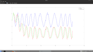
In the past I have blogged about frequency/period measurement ( e.g. here and here ) and in this post I would like to talk about a possible new way to calculate the dominant cycle period in the data. In a Stackoverflow forum post some time ago I was alerted to a recursive sinewave generator, with code, that shows how to forward generate a sine wave using just the last few values of a sine wave. It struck me that the code can be used, given the last three values of a sine wave, to calculate the period of the sine wave using simple linear regression, and in the code box below I give some Octave code which shows the basic idea.
clear all

% sine wave periods
period = input( 'Enter period: ' )
period2 = input( 'Enter period2: ' )

true_periods = [ ones( 6*period , 1 ) .* period ; ones( 3*period2 , 1 ) .* period2 ; ones( 3*period , 1 ) .* period ] ;

% create sine wave and add some noise
price = awgn( 1 .* ( 2 .+ [ sinewave( 6*period , period )' ; sinewave( 3*period2 , period2 )' ; sinewave( 3*period , period )' ] ) , 100 ) ;

% extract the signal
hp = highpass_filter_basic( price ) ;

% smooth the signal
smooth = smooth_2_5( hp ) ;

Y = smooth .+ shift( smooth , 2 ) ;
X = shift( smooth , 1 ) ;

calculated_periods = zeros( size ( price ) ) ;

% do the linear regression
for ii = 50 : size( price , 1 )
calculated_periods(ii) = ( ( X( ii-4:ii , : )' * X( ii-4:ii , : ) ) \ X( ii-4:ii , : )' ) * Y( ii-4:ii , : ) ;
end

% get the periods from regression calculations
calculated_periods = real( sqrt( ( 8 .- 4 .* calculated_periods ) ./ ( calculated_periods .+ 2 ) ) ) ;
calculated_periods = 360 ./ ( ( calculated_periods .* 180 ) ./ pi ) ;
calculated_periods = ema( calculated_periods , 3 ) ;
calculated_periods = round( calculated_periods ) ;

figure(1) ; plot( price , 'b' , "linewidth" , 2 , hp , 'r' , "linewidth" , 2 , smooth , 'g' , "linewidth" , 2 ) ; legend( 'Price' , 'Highpass' , 'Highpass smooth' ) ;
figure(2) ; plot( true_periods , 'b' , "linewidth" , 2 , calculated_periods , 'r' , "linewidth", 2 ) ; legend( 'True Periods' , 'Calculated Periods' ) ;which shows the underlying "price" in blue and the high pass filtered and smoothed versions in red and green and
shows the true and measured periods. Noisy price versions of the above are :-
and
Theoretically it seems to work, but I would like to see if things can be improved. More in my next post.


No comments:
Post a Comment