PositionBook Chart Example Trade

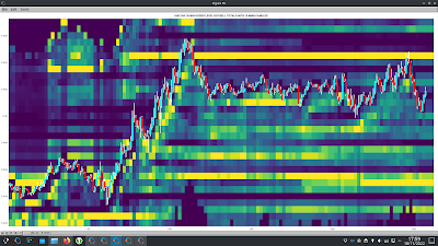
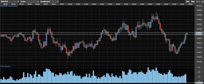
As a quick follow up to my previous post I thought I'd show an example of how one could possibly use my new PositionBook chart as a trade set-up. Below is the USD_CHF forex pair for the last two days

showing the nice run-up yesterday and then the narrow range of Friday's Asian session.

The tentative set-up idea is to look for such a narrow range and use the colour of the PositionBook chart in this range (blue for a long) to catch or anticipate a breakout. The take profit target would be the resistance suggested by the horizontal yellow bar in the open orders chart (overhead sell orders) more or less at Thursday's high.

I decided to take a really small punt on this idea but took a small loss of 0.0046 GBP

as indicated in the above Oanda trade app. I entered too soon and perhaps should have waited for confirmation (I can see a doji bar on the 5 minute chart just after my stop out) or had the conviction to re-enter the trade after this doji bar. The initial trade idea seems to have been sound as the profit target was eventually hit. This could have been a nice 4/5/6 R-multiple profitable trade.😞

A New PositionBook Chart Type

It has been almost 6 months since I last posted, due to working on a house renovation. However, I have still been thinking about/working on stuff, particularly on analysis of open position ratios. I had tried using this data as features for machine learning, but my thinking has evolved somewhat and I have reduced my ambition/expectation for this type of data.

Before I get into this I'd like to mention Trader Dale (I have no affiliation with him) as I have recently been following his volume profile set-ups, a screenshot of one being shown below.

This shows recent Wednesday action in the EUR_GBP pair on a 30 minute chart. The flexible volume profile set-up Trader Dale describes is called a Volume Accumulation Set-up which occurs immediately prior to a big break (in this case up). The whole premise of this particular set-up is that the volume accumulation area will be future support, off of which price will bounce, as shown by the "hand drawn" lines. Below is shown my version of the above chart

with a bit of extra price action included. The horizontal yellow lines show the support area.

Now here is the same data, but in what I'm calling a PositionBook chart, which uses Oanda's Position Level data downloaded via their API.

The blue (red) horizontal lines show the levels at which traders are net long (short) in terms of positions actually entered/held. The brighter the colours the greater the difference between the longs/shorts. It is obvious that the volume accumulation set-up area is showing a net accumulation of long positions and this is an indication of the direction of the anticipated breakout long before it happens. The Trader Dale set-up presumes an accumulation of longs because of the resultant breakout direction and doesn't seem to provide an opportunity to participate in the breakout itself!

The next chart shows the action of the following day and a bit where the price does indeed come back down to the "support" area but doesn't result in an immediate bounce off the support level. The following order level chart perhaps shows why there was no bounce - the relative absence of open orders at that level.

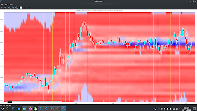
The equivalent PositionBook chart, including a bit more price action,

shows that after price fails to bounce off the support level it does recover back into it and then even more long positions are accumulated (the darker blue shade) at the support level during the London open, again allowing one to position oneself for the ensuing rise during the London morning session, followed by another long accumulation during the New York opening session for a following leg up into the London close (the last vertical red line).

This purpose of this post is not to criticise the Trader Dale set-up but rather to highlight the potential value-add of these new PositionBook charts. They seem to hold promise for indicating price direction and I intend to continue investigating/improving them in the coming weeks.

More in due course.

Simple Machine Learning Models on OrderBook/PositionBook Features

This post is about using OrderBook/PositionBook features as input to simple machine learning models after previous investigation into the relevance of such features. 

Due to the amount of training data available I decided to look only at a linear model and small neural networks (NN) with a single hidden layer with up to 6 hidden neurons. This choice was motivated by an academic paper I read online about linear models which stated that, as a lower bound, one should have at least 10 training examples for each parameter to be estimated. Other online reading about order flow imbalance (OFI) suggested there is a linear relationship between OFI and price movement. Use of limited size NNs would allow a small amount of non linearity in the relationship. For this investigation I used the Netlab toolbox and Octave. A plot of the learning curves of the classification models tested is shown below. The targets were binary 1/0 for price increases/decreases.

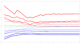
The blue lines show the average training error (y axis) and the red lines show the same average error metric on the held out cross validation data set for each tested model. The thickness of the lines represents the number of neurons in the single hidden layer of the NNs (the thicker the lines, the higher the number of hidden neurons). The horizontal green line shows the error of a generalized linear model (GLM) trained using iteratively reweighted least squares. It can be seen that NN models with 1 and 2 hidden neurons slightly outperform the GLM, with the 2 neuron model having the edge over the 1 neuron model. NN models with 3 or more hidden neurons over fit and underperform the GLM. The NN models were trained using Netlab's functions for Bayesian regularization over the parameters.

Looking at these results it would seem that a 2 neuron NN would be the best choice; however the error differences between the 1 and 2 neuron NNs and GLM are small enough to anticipate that the final classifications (with a basic greater/less than a 0.5 logistic threshold value for long/short) would perhaps be almost identical. 

Investigations into this will be the subject of my next post. 

The code box below gives the working Octave code for the above.

## load data
##training_data = dlmread( 'raw_netlab_training_features' ) ;
##cv_data = dlmread( 'raw_netlab_cv_features' ) ;
training_data = dlmread( 'netlab_training_features_svd' ) ;
cv_data = dlmread( 'netlab_cv_features_svd' ) ;
training_targets = dlmread( 'netlab_training_targets' ) ;
cv_targets = dlmread( 'netlab_cv_targets' ) ;

kk_loop_record = zeros( 30 , 7 ) ;

for kk = 1 : 30
  
## first train a glm model as a base comparison
input_dim = size( training_data , 2 ) ; ## Number of inputs.

net_lin = glm( input_dim , 1 , 'logistic' ) ; ## Create a generalized linear model structure.
options = foptions ; ## Sets default parameters for optimisation routines, for compatibility with MATLAB's foptions()
options(1) = 1 ;  ## change default value
##	OPTIONS(1) is set to 1 to display error values during training. If
##	OPTIONS(1) is set to 0, then only warning messages are displayed.  If
##	OPTIONS(1) is -1, then nothing is displayed.
options(14) = 5 ; ## change default value
##	OPTIONS(14) is the maximum number of iterations for the IRLS
##	algorithm;  default 100.
net_lin = glmtrain( net_lin , options , training_data , training_targets ) ;

## test on cv_data
glm_out = glmfwd( net_lin , cv_data ) ;
## cross-entrophy loss
glm_out_loss = -mean( cv_targets .* log( glm_out )  .+ ( 1 .- cv_targets ) .* log( 1 .- glm_out ) ) ;

kk_loop_record( kk , 7 ) = glm_out_loss ;

## now train an mlp
## Set up vector of options for the optimiser.
nouter = 30 ; ## Number of outer loops.
ninner = 2 ;	## Number of innter loops.
options = foptions ; ## Default options vector.
options( 1 ) = 1 ;	## This provides display of error values.
options( 2 ) = 1.0e-5 ; ## Absolute precision for weights.
options( 3 ) = 1.0e-5 ; ## Precision for objective function.
options( 14 ) = 100 ; ## Number of training cycles in inner loop.

training_learning_curve = zeros( nouter , 6 ) ; 
cv_learning_curve = zeros( nouter , 6 ) ;

for jj = 1 : 6

## Set up network parameters.
nin = size( training_data , 2 ) ; ## Number of inputs.
nhidden = jj ;	## Number of hidden units.
nout = 1 ; ## Number of outputs.
alpha = 0.01 ; ## Initial prior hyperparameter.
aw1 = 0.01 ;
ab1 = 0.01 ;
aw2 = 0.01 ;
ab2 = 0.01 ;

## Create and initialize network weight vector.
prior = mlpprior(nin , nhidden , nout , aw1 , ab1 , aw2 , ab2 ) ;
net = mlp( nin , nhidden , nout , 'logistic' , prior ) ;

## Train using scaled conjugate gradients, re-estimating alpha and beta.
for ii = 1 : nouter
  ## train net
  net = netopt( net , options , training_data , training_targets , 'scg' ) ;
  
  train_out = mlpfwd( net , training_data ) ;
  ## get train error
  ## mse
  ##training_learning_curve( ii ) = mean( ( training_targets .- train_out ).^2 ) ;
  
  ## cross entropy loss
  training_learning_curve( ii , jj ) = -mean( training_targets .* log( train_out )  .+ ( 1 .- training_targets ) .* log( 1 .- train_out ) ) ; 

  cv_out = mlpfwd( net , cv_data ) ;
  ## get cv error
  ## mse
  ##cv_learning_curve( ii ) = mean( ( cv_targets .- cv_out ).^2 ) ;
  
  ## cross entropy loss
  cv_learning_curve( ii , jj ) = -mean( cv_targets .* log( cv_out )  .+ ( 1 .- cv_targets ) .* log( 1 .- cv_out ) ) ; 
  
  ## now update hyperparameters based on evidence
  [ net , gamma ] = evidence( net , training_data , training_targets , ninner ) ;
  
##  fprintf( 1 , '\nRe-estimation cycle ##d:\n' , ii ) ;
##  disp( [ '  alpha = ' , num2str( net.alpha' ) ] ) ;
##  fprintf( 1 , '  gamma =  %8.5f\n\n' , gamma ) ;
##  disp(' ')
##  disp('Press any key to continue.')
  ##pause;
endfor ## ii loop

endfor ## jj loop

kk_loop_record( kk , 1 : 6 ) = cv_learning_curve( end , : ) ;

endfor ## kk loop

plot( training_learning_curve(:,1) , 'b' , 'linewidth' , 1 , cv_learning_curve(:,1) , 'r' , 'linewidth' , 1 , ...
training_learning_curve(:,2) , 'b' , 'linewidth' , 2 , cv_learning_curve(:,2) , 'r' , 'linewidth' , 2 , ...
training_learning_curve(:,3) , 'b' , 'linewidth' , 3 , cv_learning_curve(:,3) , 'r' , 'linewidth' , 3 , ...
training_learning_curve(:,4) , 'b' , 'linewidth' , 4 , cv_learning_curve(:,4) , 'r' , 'linewidth' , 4 , ...
training_learning_curve(:,5) , 'b' , 'linewidth' , 5 , cv_learning_curve(:,5) , 'r' , 'linewidth' , 5 , ...
training_learning_curve(:,6) , 'b' , 'linewidth' , 6 , cv_learning_curve(:,6) , 'r' , 'linewidth' , 6 , ...
ones( size( training_learning_curve , 1 ) , 1 ).*glm_out_loss , 'g' , 'linewidth', 2 ) ;

##  >> mean(kk_loop_record)
##  ans =
##
##     0.6928   0.6927   0.7261   0.7509   0.7821   0.8112   0.6990

##  >> std(kk_loop_record)
##  ans =
##
##     8.5241e-06   7.2869e-06   1.2999e-02   1.5285e-02   2.5769e-02   2.6844e-02   2.2584e-16

OrderBook and PositionBook Features

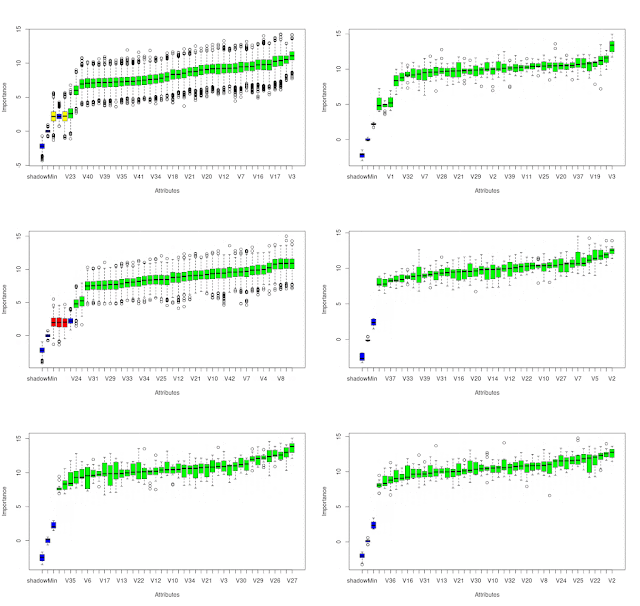
In my previous post I talked about how I planned to use constrained optimization to create features from Oanda's OrderBook and PositionBook data, which can be downloaded via their API. In addition to this I have also created a set of features based on the idea of Order Flow Imbalance (OFI), a nice exposition of which is given in this blog post along with a numerical example of how to calculate OFI. Of course Oanda's OrderBook/PositionBook data is not exactly the same as a conventional limit order book, but I thought they are similar enough to investigate using OFI on them. The result of these investigations is shown in the animated GIF below.

This shows the output from using the R Boruta package to check for the feature relevance of OFI levels to a depth of 20 of both the OrderBook and PositionBook to classify the sign of the log return of price over the periods detailed below following an OrderBook/PositionBook update (the granularity at which the OrderBook/PositionBook data can be updated is 20 minutes):

• 20 minutes
• 40 minutes
• 60 minutes
• the 20 minutes starting 20 minutes in the future
• the 20 minutes starting 40 minutes in the future

for both the OrderBook and PositionBook, giving a total of 10 separate images/results in the above GIF.

 

Observant readers may notice that in the GIF there are 42 features being checked, but only an OFI depth of 20. The reason for this is that the data contain information about buys/sell orders and long/short positions both above and below the current price, so what I did was calculate OFI for:

• buy orders above price vs sell orders below price
• sell orders above price vs buy orders below price
• long positions above price vs short positions below price
• short positions above price vs long positions below price 

As can be seen, almost all features are deemed to be relevant with the exception of 3 OFI levels rejected (red candles) and 2 deemed tentative (yellow candles).

It is my intention to use these features in a machine learning model to classify the probability of future market direction over the time frames mentioned above. 

More in due course.

A Possible, New Positionbook Indicator?

In my previous post I ended with saying that I would post about some sort of "sentiment indicator" if, and only if, I had something positive to say about my progress on this work. This post is the first on this subject.

The indicator I'm working on is based on the open position ratios data that is available via the Oanda api. For the uninitiated, this data gives the percentage of traders holding long and short positions, and at what price levels, in 14 selected forex pairs and also gold and silver. The data is updated every 20 minutes. I have long felt that there must be some value hidden in this data but the problem is how to extract it.

What I've done is take the percentage values from the (usually) hundreds of separate price levels and sum and normalise them over three defined ranges - levels above/below the high/low of each 20 minute period and the level(s) that span the price range of this period. This is done separately for long and short positions to give a total of 6 percentage figures that sum to 100%. Conceptually, this can be thought of as attaching to the open and close of a 20 minute OHLC bar the 6 percentage position values that were in force at the open and close respectively. The problem is to try and infer the actual, net changes in positions that have taken place over the time period this 20 minute bar was forming. In this way I am trying, if you like, to create a sort of  "skin in the game" indicator as opposed to an indicator derived from order book data, which could be said to be based on traders' current (changeable) intentions as expressed by their open orders and which are subject to shenanigans such as spoofing.

The methodology I've decided on to realise the above is constrained optimization using Octave's fmincon function. The objective function is simply:

    denom = X' * old_pb_net_pos ;
    J = mean( ( new_pb_net_pos .- ( ( X .* old_pb_net_pos ) ./ denom ) ).^2 ) ;

for a multiplicative position value change model where:

• X is a vector of constants that are to be optimised
• old_pb_net_pos is a vector of the 6 percentage values at the open
• new_pb_net_pos is a vector of the 6 percentage values at the close

This is a constrained model because percentage position values at price levels outside the bar range cannot actually increase as a result of trades that take place within the bar range, so the X values for these levels are necessarily constrained to a maximum value of 1 (implying no real, absolute change at these levels). Similarly, all X values must be greater than zero (a zero value would imply a mass exit of all positions at this level, which never actually happens).

The net result of the above is an optimised X vector consisting of multiplicative constants that are multiplied with old_pb_net_pos to achieve new_pb_net_pos according to the logic exemplified in the above objective function. It is these optimised X values from which the underlying, real changes in positions will be inferred and features created. More on this in my next post.

 

Matrix Profile and Weakly Labelled Data - 2nd and Final Update

It has been over three months since my last post, which was intended to be the first in a series of posts on the subject of the title of this post. However, it turned out that the results of my work were underwhelming and so I decided to stop flogging a dead horse and move onto other things. I still have some ideas for using Matrix Profile, but not for the above. These ideas may be the subject of a future blog post.

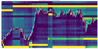
I subsequently looked at plotting order levels using the data that is available via the Oanda API and I have come up with Octave code to render plots such as this:

where the brighter yellow stripes show ranges where there is an accumulation of sell/buy orders above/below price. These can be interpreted as support/resistance areas. It is normally my practice to post my Octave code, but the code for this plot is quite idiosyncratic and depends very much on the way I have chosen to store the underlying data downloaded from Oanda. As such, I don't think it would be helpful to readers and so I am not posting the code. That said, if there is actually a demand I am more than happy to make it available in a future blog post.

Having done this, it seemed natural to extend it to Open Position Ratios which are also available via the Oanda API. Plotting these levels renders plots that are similar to the plot shown above, but show levels where open long/short positions instead of open orders are accumulated. Although such plots are visually informative, I prefer something more objective, and so for the last few weeks I have been working on using the open position ratios data to construct some sort of sentiment indicator that hopefully could give a heads up to future price movement direction. This is still very much a work in progress which I shall post about if there are noteworthy results.

More in due course.