Judging the Quality of Indicators.

In my previous post I said I was trying to develop new indicators from the results of my new PositionBook optimisation routine. In doing so, I need to have a methodology for judging the quality of the indicator(s). In the past I created a Data-Snooping-Tests-GitHub which contains some tests for statistical significance testing and which, of course, can be used on these new indicators. Additionally, for many years I have had a link to tssb on this blog from where a free testing program, VarScreen, and its associated manual are available. Timothy Masters also has a book, Testing and Tuning Market Trading Systems, wherein there is C++ code for an Entropy test, an Octave compiled .oct version of which is shown in the following code box.

#include "octave oct.h"
#include "octave dcolvector.h"
#include "cmath"
#include "algorithm"

DEFUN_DLD ( entropy, args, nargout,
"-*- texinfo -*-\n\
@deftypefn {Function File} {entropy_value =} entropy (@var{input_vector,nbins})\n\
This function takes an input vector and nbins and calculates\n\
the entropy of the input_vector. This input_vector will usually\n\
be an indicator for which we want the entropy value. This value ranges\n\
from 0 to 1 and a minimum value of 0.5 is recommended. Less than 0.1 is\n\
serious and should be addressed. If nbins is not supplied, a default value\n\
of 20 is used. If the input_vector length is < 50, an error will be thrown.\n\
@end deftypefn" )

{
octave_value_list retval_list ;
int nargin = args.length () ;
int nbins , k ;
double entropy , factor , p , sum ;

// check the input arguments
if ( args(0).length () < 50 )
   {
   error ("Invalid 1st argument length. Input is a vector of length >= 50.") ;
   return retval_list ;
   }

if ( nargin == 1 )
   {
   nbins = 20 ;
   }

if ( nargin == 2 )
   {
   nbins = args(1).int_value() ;
   }
// end of input checking

ColumnVector input = args(0).column_vector_value () ;
ColumnVector count( nbins ) ;
double max_val = *std::max_element( &input(0), &input( args(0).length () - 1 ) ) ;
double min_val = *std::min_element( &input(0), &input( args(0).length () - 1 ) ) ;
factor = ( nbins - 1.e-10 ) / ( max_val - min_val + 1.e-60 ) ;

for ( octave_idx_type ii ( 0 ) ; ii < args(0).length () ; ii++ ) {
      k = ( int ) ( factor * ( input( ii ) - min_val ) ) ;
      ++count( k ) ; }

sum = 0.0 ;
for ( octave_idx_type ii ( 0 ) ; ii < nbins ; ii++ ) {
      if ( count( ii ) ) {
         p = ( double ) count( ii ) / args(0).length () ;
        sum += p * log ( p ) ; }
        }

entropy = -sum / log ( (double) nbins ) ;

retval_list( 0 ) = entropy ;

return retval_list ;

} // end of function

This calculates the information content, Entropy_(information_theory), of any indicator, the value for which ranges from 0 to 1, with a value of 1 being ideal. Masters suggests that a minimum value of 0.5 is acceptable for indicators and also suggests ways in which the calculation of any indicator can be adjusted to improve its entropy value. By way of example, below is a plot of an "ideal" (blue) indicator, which has values uniformly spread across its range

with an entropy value of 0.9998. This second plot shows a "good" indicator, which has an

entropy value of 0.7781 and is in fact just random, normally distributed values with a mean of 0 and variance 1. In both plots, the red indicators fail to meet the recommended minimum value, both having entropy values of 0.2314.

It is visually intuitive that in both plots the blue indicators convey more information than the red ones. In creating my new PositionBook indicators I intend to construct them in such a way as to maximise their entropy before I progress to some of the above mentioned tests.

Update to PositionBook Chart - Revised Optimisation Method

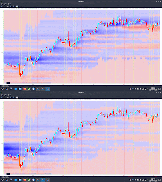
Just over a year ago I previewed a new chart type which I called a "PositionBook Chart" and gave examples in this post and this one. These first examples were based on an optimisation routine over 6 variables using Octave's fminunc function, an unconstrained minimisation routine. However, I was not 100% convinced that the model I was using for the loss/cost function was realistic, and so since the above posts I have been further testing different models to see if I could come up with a more satisfactory model and optimisation routine. The comparison between the original model and the better, newer model I have selected is indicated in the following animated GIF, which shows the last few day's action in the GBPUSD forex pair. 

The old model is figure(200), with the darker blue "blob" of positions accumulated at the lower, beginning of the chart, and the newer model, figure(900), shows accumulation throughout the uptrend. The reasons I prefer this newer model are:

• 4 of the 6 variables mentioned above (longs above and below price bar range, and shorts above and below price bar range) are theoretically linked to each other to preserve their mutual relationships and jointly minimised over a single input to the loss/cost function, which has a bounded upper and lower limit. This means I can use Octave's fminbnd function instead of fminunc. The minimisation objective is the minimum absolute change in positions outside the price bar range, which has a real world relevance as compared to the mean squared error of the fminunc cost function.
• because fminunc is "unconstrained" occasionally it would converge to unrealistic solutions with respect to position changes outside the price bar range. This does not happen with the new routine.
• once the results of fminbnd are obtained, it is possible to mathematically calculate the position changes within the price bar range exactly, without needing to resort to any optimisation routine. This gives a zero error for the change which is arguably the most important.
• the results from the new routine seem to be more stable in that indicators I am trying to create from them are noticeably less erratic and confusing than those created from fminunc results.
• finally, fminbnd over 1 variable is much quicker to converge than fminunc over 6 variables.
  

The second last mentioned point, derived indicators, will be the subject of my next post.

Currency Strength Revisited

Recently I responded to a Quantitative Finance forum question here, where I invited the questioner to peruse certain posts on this blog. Apparently the posts do not provide enough information to fully answer the question (my bad) and therefore this post provides what I think will suffice as a full and complete reply, although perhaps not scientifically rigorous.

The original question asked was "Is it possible to separate or decouple the two currencies in a trading pair?" and I believe what I have previously described as a "currency strength indicator" does precisely this (blog search term ---> https://dekalogblog.blogspot.com/search?q=currency+strength+indicator). This post outlines the rationale behind my approach.

Take, for example, the GBPUSD forex pair, and further give it a current (imaginary) value of 1.2500. What does this mean? Of course it means 1 GBP will currently buy you 1.25 USD, or alternatively 1 USD will buy you 1/1.25 = 0.8 GBP. Now rather than write GBPUSD let's express GBPUSD as a ratio thus:- GBP/USD, which expresses the idea of "how many USD are there in a GBP?" in the same way that 9/3 shows how many 3s there are in 9. Now let's imagine at some time period later there is a new pair value, a lower case "gbp/usd" where we can write the relationship

                    (1)     ( GBP / USD ) * ( G / U ) = gbp / usd

to show the change over the time period in question. The ( G / U ) term is a multiplicative term to show the change in value from old GBP/USD 1.2500 to say new value gbp/usd of 1.2600, 

e.g.                ( G / U ) == ( gbp / usd ) / ( GBP / USD ) == 1.26 / 1.25 == 1.008

from which it is clear that the forex pair has increased by 0.8% in value over this time period. Now, if we imagine that over this time period the underlying, real value of USD has remained unchanged this is equivalent to setting the value U in ( G / U ) to exactly 1, thereby implying that the 0.8% increase in the forex pair value is entirely attributable to a 0.8% increase in the underlying, real value of GBP, i.e. G == 1.008. Alternatively, we can assume that the value of GBP remains unchanged,

 e.g.                G == 1, which means that U == 1 / 1.008 == 0.9921

which implies that a ( 1 - 0.9921 ) == 0.79% decrease in USD value is responsible for the 0.8% increase in the pair quote.

Of course, given only equation (1) it is impossible to solve for G and U as either can be arbitrarily set to any number greater than zero and then be compensated for by setting the other number such that the constant ( G / U ) will match the required constant to account for the change in the pair value.

However, now let's introduce two other forex pairs (2) and (3) and thus we have:-

                    (1)     ( GBP / USD ) * ( G / U ) = gbp / usd

                    (2)     ( EUR / USD ) * ( E / U ) = eur / usd

                    (3)     ( EUR / GBP ) * ( E / G ) = eur / gbp

We now have three equations and three unknowns, namely G, E and U, and so this system of equations could be laboriously, mathematically solved by substitution. 

However, in my currency strength indicator I have taken a different approach. Instead of solving mathematically I have written an error function which takes as arguments a list of G, E, U, ... etc. for all currency multipliers relevant to all the forex quotes I have access to, approximately 47 various crosses which themselves are inputs to the error function, and this function is supplied to Octave's fminunc function to simultaneously solve for all G, E, U, ... etc. given all forex market quotes. The initial starting values for all G, E, U, ... etc. are 1, implying no change in values across the market. These starting values consistently converge to the same final values for G, E, U, ... etc for each separate period's optimisation iterations.

Having got all G, E, U, ... etc. what can be done? Well, taking G for example, we can write

                    (4)     GBP * G = gbp

for the underlying, real change in the value of GBP. Dividing each side of (4) by GBP and taking logs we get

                    (5)     log( G ) = log( gbp / GBP )

i.e. the log of the fminunc returned value for the multiplicative constant G is the equivalent of the log return of GBP independent of all other currencies, or as the original forum question asked, the (change in) value of GBP separated or decoupled the from the pair in which it is quoted.

Of course, having the individual log returns of separated or decoupled currencies, there are many things that can be done with them, such as:-

• create indices for each currency
• apply technical analysis to these separate indices
• intermarket currency analysis
• input to machine learning (ML) models
• possibly create new and unique currency indicators

Examples of the creation of "alternative price charts" and indices are shown below

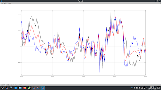
where the black line is the actual 10 minute closing prices of GBPUSD over the last week (13th to 18th August) with the corresponding GBP price (blue line) being the "alternative" GBPUSD chart if U is held at 1 in the ( G / U ) term and G allowed to be its derived, optimised value, and the USD price (red line) being the alternative chart if G is held at 1 and U allowed to be its derived, optimised value.

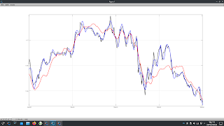
This second chart shows a more "traditional" index like chart

where the starting values are 1 and both the G and U values take their derived values. As can be seen, over the week there was upwards momentum in both the GBP and USD, with the greater momentum being in the GBP resulting in a higher GBPUSD quote at the end of the week. If, in the second chart the blue GBP line had been flat at a value of 1 all week, the upwards momentum in USD would have resulted in a lower week ending quoted value of GBPUSD, as seen in the red USD line in the first chart. Having access to these real, decoupled returns allows one to see through the given, quoted forex prices in the manner of viewing the market as though through X-ray vision. 

I hope readers find this post enlightening, and if you find some other uses for this idea, I would be interested in hearing how you use it.
 

Quick Update on Kalman Filter and Sensor Fusion

Managed to code it up and get it working, but at the end of the day I couldn't see any value added over just averaging the output of the indicators I was trying to fuse together via Kalman filtering. As a result, I'm giving up on this for now and looking at other things.

More in due course. 

Kalman Filter and Sensor Fusion.

In the Spring of 2012 and again in the Spring of 2019 I posted a series of posts about the Kalman Filter, which readers can access via the blog archive on the right. In both cases I eventually gave up those particular lines of investigation because of disappointing results. This post is the first in a new series about using the Kalman Filter for sensor fusion, which I had known of before, but due to the paucity of clear information about this online I had never really investigated. However, my recent discovery of this Github and its associated online tutorial has inspired me to a third attempt at using Kalman Filters. What I am going to attempt to do is use the idea of sensor fusion to fuse the output of several functions I have coded in the past, which each extract the dominant cycle from a time series, to hopefully obtain a better representation of the "true underlying cycle."

The first step in this process is to determine the measurement noise covariance or, in Kalman Filter terms, the "R" covariance matrix. To do this, I have used the average of two of the outputs from the above mentioned functions to create a new cycle and similarly used two extracted trends (price minus these cycles) averaged to get a new trend. The new cycle and new trend are simply added to each other to create a new price series which is almost identical to the original price series. The screenshot below shows a typical cycle extract,

where the red cycle is the average of the other two extracted cycles, and this following screenshot shows the new trend in red plus the new price alongside the old price (blue and black respectively).

Having created a time series thus with known trend and cycle, it is a simple matter to run my cycle extractor functions on this new price, compare the outputs with the known cyclic component of price and calculate the variance of the errors to get the R covariance matrices for 14 different currency crosses.

More in due course.