Showing posts with label Synthetic Data. Show all posts

Tuesday, 28 February 2023

Kalman Filter and Sensor Fusion.

In the Spring of 2012 and again in the Spring of 2019 I posted a series of posts about the Kalman Filter, which readers can access via the blog archive on the right. In both cases I eventually gave up those particular lines of investigation because of disappointing results. This post is the first in a new series about using the Kalman Filter for sensor fusion, which I had known of before, but due to the paucity of clear information about this online I had never really investigated. However, my recent discovery of this Github and its associated online tutorial has inspired me to a third attempt at using Kalman Filters. What I am going to attempt to do is use the idea of sensor fusion to fuse the output of several functions I have coded in the past, which each extract the dominant cycle from a time series, to hopefully obtain a better representation of the "true underlying cycle."

The first step in this process is to determine the measurement noise covariance or, in Kalman Filter terms, the "R" covariance matrix. To do this, I have used the average of two of the outputs from the above mentioned functions to create a new cycle and similarly used two extracted trends (price minus these cycles) averaged to get a new trend. The new cycle and new trend are simply added to each other to create a new price series which is almost identical to the original price series. The screenshot below shows a typical cycle extract,

where the red cycle is the average of the other two extracted cycles, and this following screenshot shows the new trend in red plus the new price alongside the old price (blue and black respectively).
Having created a time series thus with known trend and cycle, it is a simple matter to run my cycle extractor functions on this new price, compare the outputs with the known cyclic component of price and calculate the variance of the errors to get the R covariance matrices for 14 different currency crosses.

More in due course.


Thursday, 18 June 2020

More Work on RVFL Networks

Back in November last year I posted about Random Vector Functional Link (RVFL) networks here and here. Since then, along with my recent work on Oanda's API Octave functions and Market/Volume Profile visualisation, I have continued looking at RVFL networks and this post is an update on this work.

The "random" in RVFL means random initialisation of weights that are then fixed. It seems to me that it might be possible to do better than random by having some principled way of weight initialisation. To this end I have used the Penalised MATLAB Toolbox on features derived from my ideal cyclic tau embedding function to at first train a Generalized Linear Model with the Lasso penalty and then the Ridge penalty over thousands of sets of Monte Carlo generated, ideal cyclic prices and such prices with trends. The best weights for each set of prices were recorded in an array and then the mean weight (and standard deviation) taken. This set of mean weights is intended to replace the random weights in a RVFL network designed to predict the probability of "price" being at a cyclic turning point using the above cyclic tau embedding features.

Of course these weights could be considered a trained model in and of themselves, and the following screenshots show "out of sample" performance on Monte Carlo generated ideal prices that were not used in the training of the mean weights.
The black line is the underlying cyclic price and the red, blue and green lines are the mean weight model probabilities for cyclic peaks, troughs or neither respectively. Points where the peak/trough probabilities exceed the neither probabilities are marked by the red and blue vertical lines. Similarly, we have prices trending up in a cyclic fashion
and also trending down
In the cases of the last two trending markets only the swing highs and lows are indicated. The reason for this is that during training, based on my "expert knowledge" of the cyclic tau features used, it is unreasonable to expect these features to accurately capture the end of an up leg in a bull trend or the end of a down leg in a bear trend - hence these were not presented as a positive class during training.

As I said above the motivation for this is to get a more meaningful hidden layer in a RVFL network. This hidden layer will consist of seven Sigmoid functions which each give a probability of price being at or not being at a cyclic turn, conditional upon the type of market the input weights were trained on.

More in due course.

Wednesday, 30 October 2019

Weight Agnostic Neural Net Training

I have recently come across the idea of weight agnostic neural net training and have implemented a crude version of this combined with the recent work I have been doing on Taken's Theorem ( see my posts here, here and here ) and using the statistical mechanics approach to creating synthetic data.

Using the simple Octave function below with the Akaike Information Criterion as the minimisation objective
## Copyright (C) 2019 dekalog
## 
## This program is free software: you can redistribute it and/or modify it
## under the terms of the GNU General Public License as published by
## the Free Software Foundation, either version 3 of the License, or
## (at your option) any later version.
## 
## This program is distributed in the hope that it will be useful, but
## WITHOUT ANY WARRANTY; without even the implied warranty of
## MERCHANTABILITY or FITNESS FOR A PARTICULAR PURPOSE.  See the
## GNU General Public License for more details.
## 
## You should have received a copy of the GNU General Public License
## along with this program.  If not, see
## .

## -*- texinfo -*- 
## @deftypefn {} {@var{J} =} wann_training_of_cyclic_embedding()
##
## @seealso{}
## @end deftypefn

## Author: dekalog 
## Created: 2019-10-26

function J = wann_training_of_cyclic_embedding( x )
global sample_features ; global sample_targets ;
epsilon = 1e-15 ; ## to ensure log() does not give out a nan

## get the parameters from input x
activation_funcs = floor( x( 1 : 5 ) ) ; ## get the activations, 1 == sigmoid, 2 == tanh, 3 == Lecun sigmoid
layer_size = floor( x( 6 : 10 ) ) ;

[ min_layer_size , ix_min ] = min( layer_size ) ;
  if( min_layer_size > 0 ) ## to be expected most of the time
    nn_depth = length( layer_size ) ;
  elseif( min_layer_size == 0 ) ## one layer has no nodes, hence limits depth of nn
    nn_depth = ix_min - 1 ;
  endif 

length_jj_loop = 25 ;
all_aic_values = zeros( length_jj_loop , 1 ) ;  
  
for jj = 1 : length_jj_loop 
  
  previous_layer_out = sample_features ;
  sum_of_k = 0 ;
    
  for ii = 1 : nn_depth
    
    new_weight_matrix = ones( size( previous_layer_out , 2 ) , layer_size( ii ) ) ./ sqrt( size( previous_layer_out , 2 ) ) ;
    sum_of_k = sum_of_k + numel( new_weight_matrix ) ;
    prior_to_activation_input = previous_layer_out * new_weight_matrix ;

    ## select the activation function 
    if( activation_funcs( ii ) == 1 ) ## sigmoid activation
      previous_layer_out = 1.0 ./ ( 1.0 .+ exp( -prior_to_activation_input ) ) ;
    elseif( activation_funcs( ii ) == 2 ) ## tanh activation
      previous_layer_out = tanh( prior_to_activation_input ) ;
    elseif( activation_funcs( ii ) == 3 ) ## lecun sigmoid activation
      previous_layer_out = sigmoid_lecun_m( prior_to_activation_input ) ;
    endif 
    
  endfor

  ## the final logistic output
  new_weight_matrix = ones( size( previous_layer_out , 2 ) , 1 ) ./ sqrt( size( previous_layer_out , 2 ) ) ;
  sum_of_k = sum_of_k + numel( new_weight_matrix ) ;
  final_output = previous_layer_out * new_weight_matrix ;
  final_output = 1.0 ./ ( 1.0 .+ exp( -final_output ) ) ;

  max_likelihood = sum( log( final_output .+ epsilon ) .* sample_targets + log( 1 .- final_output .+ epsilon ) .* ( 1 .- sample_targets ) ) ;
  
  ## get Akaike Information criteria
  all_aic_values( jj ) = 2 * sum_of_k - 2 * max_likelihood ;

endfor ## end of jj loop

J = mean( all_aic_values ) ;

endfunction
and the Octave interface of the Bayesopt Library I am currently iterating over different architectures ( up to 5 hidden layers deep with a max of 100 nodes per layer and using a choice of 3 hidden activations ) for a simple Logistic Regression model to predict turning points in different sets of statistical mechanics synthetic data using just features based on Taken's embedding.

More in due course.

Saturday, 12 October 2019

Another Method of Creating Synthetic Data

Over the years I have posted about several different methodologies for creating synthetic data and I have recently come across yet another one which readers may find useful.

One of my first posts was Creation of Synthetic Data, which essentially is a random scrambling of historic data for a single time series with an attempt to preserve some of the bar to bar dependencies based upon a bar's position in relation to upper and lower price envelopes, a la Bollinger Bands, although the code provided in this post doesn't actually use Bollinger Bands. Another post, Creating Synthetic Data Using the Fast Fourier Transform, randomly scrambles data in the frequency domain.

Rather than random scrambling of existing data, another approach is to take measurements from existing data and then use these measurements to recreate new data series with similar characteristics. My Hidden Markov Modelling of Synthetic Periodic Time Series Data post utilises this approach and can be used to superimpose known sinusoidal waveforms onto historical trends. The resultant synthetic data can be used, as I have used it, in a form of controlled experiment whereby indicators etc. can be measured against known cyclic prices.

All of the above share the fact that they are applied to univariate time series only, although I have no doubt that they could probably be extended to the multivariate case. However, the new methodology I have come across is Statistical Mechanics of Time Series and its matlab central file exchange "toolbox." My use of this is to produce ensembles of my Currency Strength Indicator, from which I am now able to produce 50/60+ separate, synthetic time series representing, for example, all the Forex pairs, and preserving their inter-relationships whilst only suffering the computational burden of applying this methodology to a dozen or so underlying "fundamental" time series.

This may very well become my "go to" methodology for generating unlimited amounts of training data.

Monday, 16 September 2019

The Ideal Tau for Time Series Embedding?

In my Preliminary Test Results of Time Series Embedding post I got a bit ahead of myself and mistakenly quoted the ideal embedding length (Tau) to be half a period for cyclic prices. This should actually have been a quarter of a period and I have now corrected my earlier post.

This post is about my further investigations, which uncovered the above, and is written in a logical progression rather than the order in which I actually did things.

It was important to look at the Tau value for ideal sinusoidal data to confirm the quarter period, which checked out because I was able to easily recreate the 2D Lissajous curves in the Novel Method for Topological Embedding of Time-Series Data paper. I then extended this approach to 3D to produce plots such as this one, which may require some explaining.
This is a 3D Phase space plot of adaptive Max Min Normalised "sinusoidal prices" normalised to fall in the range [ -1 +1 ] and adaptive to the known, underlying period of the sine wave. This was done for prices with and without a "trend." The circular orbits are for the pure sine wave, representing cyclic price action plotted in 3D as current price, price delayed by a quarter of a cycle (Tau 1) and by half a cycle (Tau 2). The mini, blue and red "constellations" outside the circular orbits are the same pure sine wave(s) with an uptrend and downtrend added. The utility of this representation for market classification etc. is obvious, but is not the focus of this post.

Looking at Tau values for ideal prices with various trends taken from real market data, normalised as described above, across a range of known periods (because they were synthetically generated) the following results were obtained.
This is a plot of periods 10 to 47 (left to right along the x-axis) vs the global tau value (y-axis) measured using my Octave version of the mdDelay.m function from the mdembedding github. Each individual, coloured line plot is based on the underlying trend of one of 66 different, real time series. Each point per period per tradeable is the median value of 20 Monte Carlo runs over that tradeable's trend + synthetic, ideal sine wave price. The thick, black line is the median of the median values per period. Although noisy, it can be seen that the median line(s) straddle the theoretical, quarter cycle Tau (0.25) quite nicely. It should be remembered that this is on normalised prices. For comparison, the below plot shows the same on the unnormalised prices.
where the Tau value starts at over 0.5 at a cyclic period of 10 at the left and then slowly decreases to just over 0.1 at period 47.

More in due course.

Thursday, 5 September 2019

Preliminary Test Results of Time Series Embedding

Following on from my post yesterday, this post presents some preliminary results from the test I was running while writing yesterday's post. However, before I get to these results I would like to talk a bit about the hypothesis being tested.

I had an inkling that the dominant cycle period might having some bearing on tau, the time delay for the time series embedding implied by Taken's theorem, so I set up the test (described below) and after writing the post yesterday, and while the test was still running, I did some online research to see if there is any theoretical justification available.

One of the papers I found online is A Novel Method for Topological Embedding of Time-Series Data. From the abstract

"...we propose a novel method for embedding one-dimensional, periodic time-series data into higher-dimensional topological spaces to support robust recovery of signal features via topological data analysis under noisy sampling conditions...To provide evidence for the viability of this method, we analyze the simple case of sinusoidal data..."

One of the conclusions drawn is that for sinusoidal data the ideal embedding length is a quarter of the cycle period, i.e. Π/2.

Another paper I found was Topological time-series analysis with delay-variant embedding. This paper investigates "delay-variant embedding," essentially making the embedding length tau variable. From the concluding remarks

"We have demonstrated that the topological features that are constructed using delay-variant embedding can capture the topological variation in a time series when the time-delay value changes... These results indicate that the topological features that are deduced with delay-variant embedding can be used to reveal the representative features of the original time series."

My inkling was that tau should be adaptive to the measured dominant cycle, and both the above linked papers do provide some justification. Anyway, on to the test.

Reusing the code from my earlier post here I created synthetic price series with known but variable dominant cycle periods and based on real price trends, which results in synthetic series that are highly correlated with real price series but with underlying characteristics being exactly known. I then used my version of mdembedding code to calculate tau for numerous Monte Carlo replications of time series of prices based on a range of real forex pairs prices, gold and silver prices and different indices created by my currency strength indicator methodology. I then created a ratio of tau/average_measured_period measured as a global value across the whole of each individual time series replication as the test statistic, with the period being measured by an autocorrelation periodogram function: a ratio value of 0.5, for example, meaning that the tau for that time series is half the average period over the whole series.

Below is a plot of the histogram of these ratios:
which shows the ratios being centred approximately around 0.4 but with a long right tail. The following histogram is of the means of the bootstrap with replacement of the above distribution,
which is centred around a mean value of 0.436. Using this bootstrapped mean ratio of tau/period implies, for example, that the ideal tau for an average period of 20 is 8.72, which when rounded up to 9, is almost twice the theoretical ideal of a 5 day tau for 20 day cyclic period prices.

Personally I think this is an encouraging set of preliminary test results, with some caveats. More in due course.

Thursday, 6 June 2019

Determining the Noise Covariance Matrix R for a Kalman Filter

An important part of getting a Kalman filter to work well is tuning the process noise covariance matrix Q and the measurement noise covariance matrix R. This post is about obtaining the R matrix, with a post about the Q matrix to come in due course.

In my last post about the alternative version extended kalman filter to model a sine wave I explained that the 4 measurements are the sine wave value itself, and the phase, angular frequency and amplitude of the sine wave. The phase and angular frequencies are "measured" using outputs of the sinewave indicator and the amplitude is calculated as an RMS value over a measured period. The "problem" with this is that the accuracies of such measurements on real data are unknown, and therefore so is the R matrix, because the underlying cycle properties are unknown. My solution to this is offline Monte Carlo simulation.

As a first step the Octave code in the box immediately below
clear all ;
pkg load statistics ;

%%%%%%%%%%%%%%%%%%%%%%%%%%%%%%%%%%%%%%%%%%%%%%%%%%%%%%%%%%%%%%%%%%%%%%%%%%%%%%%%
% load data

raw_data = dlmread( 'raw_data_for_indices_and_strengths' ) ;
delete_hkd_crosses = [ 3 9 12 18 26 31 34 39 43 51 61 ] .+ 1 ; % +1 to account for date column
raw_data( : , delete_hkd_crosses ) = [] ;
raw_data( : , 1 ) = [] ; % delete data vector 

all_g_c = dlmread( "all_g_mults_c" ) ; % the currency g mults
all_g_c( : , 7 ) = [] ; % delete hkd index

all_g_s = dlmread( "all_g_sv" ) ;      % the gold and silver g mults   
all_g_c = [ all_g_c all_g_s(:,2:3) ] ; % a combination of the above 2
all_g_c( : , 2 : end ) = cumprod( all_g_c( : , 2 : end) , 1 ) ;
all_g_c( : , 1 ) = [] ; % delete date vector

all_raw_data = [ raw_data all_g_c ] ;

%%%%%%%%%%%%%%%%%%%%%%%%%%%%%%%%%%%%%%%%%%%%%%%%%%%%%%%%%%%%%%%%%%%%%%%%%%%%%%%%

% set up recording vectors
amplitude = zeros( size( all_raw_data , 1 ) , 1 ) ;
all_amplitudes = zeros( size( all_raw_data ) ) ;
all_periods = all_amplitudes ;

for ii = 1 : size( all_raw_data , 2 )
  
  price = all_raw_data( : , ii ) ;
  period = autocorrelation_periodogram( price ) ;
  all_periods( : , ii ) = period ;
  [ hp , ~ ] = highpass_filter_basic( price ) ; hp( 1 : 99 ) = 0 ;

  for jj = 100 : size( all_raw_data , 1 )
    amplitude( jj ) = sqrt( 2 ) * sqrt( mean( hp( round( jj - period( jj ) / 2 ) : jj , 1 ).^2 ) ) ;
  endfor
  
  % store information about amplitude changes as a multiplicative constant
  all_amplitudes( : , ii ) = amplitude ./ shift( amplitude , 1 ) ;

endfor

% truncate
all_amplitudes( 1 : 101 , : ) = [] ;
all_periods( 1 : 101 , : ) = [] ;

max_period = max( max( all_periods ) ) ;
min_period = min( min( all_periods ) ) ;

% unroll
all_amplitudes = all_amplitudes( : ) ; all_periods = all_periods( : ) ;

amplitude_changes = cell( max_period , 1 ) ;

for ii = min_period : max_period
  ix = find( all_periods == ii ) ;
  amplitude_changes{ ii , 1 } = all_amplitudes( ix , 1 ) ;
endfor

save all_amplitude_changes amplitude_changes ;
is used to get information about cycle amplitudes from real data and store it in a cell array.

This next box shows code that uses this cell array, plus earlier hidden markov modelling code for sine wave modelling, to produce synthetic price data
clear all ;
pkg load signal ;
pkg load statistics ;

%%%%%%%%%%%%%%%%%%%%%%%%%%%%%%%%%%%%%%%%%%%%%%%%%%%%%%%%%%%%%%%%%%%%%%%%%%%%
% load data

raw_data = dlmread( 'raw_data_for_indices_and_strengths' ) ;
delete_hkd_crosses = [ 3 9 12 18 26 31 34 39 43 51 61 ] .+ 1 ; % +1 to account for date column
raw_data( : , delete_hkd_crosses ) = [] ;
raw_data( : , 1 ) = [] ; % delete date vector
all_g_c = dlmread( "all_g_mults_c" ) ; % the currency g mults
all_g_c( : , 7 ) = [] ; % delete hkd index
all_g_s = dlmread( "all_g_sv" ) ;      % the gold and silver g mults   
all_g_c = [ all_g_c all_g_s(:,2:3) ] ; % a combination of the above 2
all_g_c( : , 2 : end ) = cumprod( all_g_c( : , 2 : end) , 1 ) ;
all_g_c( : , 1 ) = [] ; % delete date vector
all_raw_data = [ raw_data all_g_c ] ; clear -x all_raw_data ;

%%%%%%%%%%%%%%%%%%%%%%%%%%%%%%%%%%%%%%%%%%%%%%%%%%%%%%%%%%%%%%%%%%%%%%%%%%%%

load all_hmm_periods_daily ;
load all_amplitude_changes ;

% choose an ix for all_raw_data
ix = input( "ix? " ) ;
price = all_raw_data( : , ix ) ;
period = autocorrelation_periodogram( price ) ;
[ hp , trend ] = highpass_filter_basic( price ) ;

% estimate variance of cycle noise
hp_filt = sgolayfilt( hp , 2 , 7 ) ;
noise = hp( 101 : end ) .- hp_filt( 101 : end ) ; noise_var = var( noise ) ;
% zero pad beginning of noise vector
noise = [ zeros( 100 , 1 ) ; noise ] ;

% set for plotting purposes
hp( 1 : 50 ) = 0 ; trend( 1 : 50 ) = price( 1 : 50 ) ;

% create sine wave with known phase and period/angular frequency 
[ gen_period , ~ ] = hmmgenerate( length( price ) , transprobest , outprobest ) ;
gen_period = gen_period .+ hmm_min_period_add ;
phase = cumsum( ( 2 * pi ) ./ gen_period ) ; phase = mod( phase , 2 * pi ) ;
gen_sine = sin( phase ) ;

% amplitude vector
amp = ones( size( hp ) ) ;

% RMS initial amplitude 
amp( 100 ) = sqrt( 2 ) * sqrt( mean( hp( 100 - period( 100 ) : 100 ).^2 ) ) ;

% alter sine wave with known amplitude
for ii = 101 : length( hp )
  % get multiple for this period
  random_amp_mults = amplitude_changes{ gen_period( ii ) } ;
  rand_mult = random_amp_mults( randi( size( random_amp_mults , 1 ) , 1 ) ) ;
  amp( ii ) = rand_mult * sqrt( 2 ) * sqrt( mean( hp( ii - 1 - period( ii - 1 ) : ii - 1 ).^2 ) ) ; ;
  gen_sine( ii ) = amp( ii ) * gen_sine( ii ) ; 
endfor

% estimate variance of generated cycle noise
gen_filt = sgolayfilt( gen_sine , 2 , 7 ) ;
gen_noise = gen_sine( 101 : end ) .- gen_filt( 101 : end ) ; gen_noise_var = var( gen_noise ) ;

% a crude adjustment of generated cycle noise to match "real" noise by adding
% noise
gen_sine = gen_sine' .+ noise ;

% set beginning of gen_sine to real cycle for plotting purposes
gen_sine( 1 : 100 ) = hp( 1 : 100 ) ;
new_price = trend .+ gen_sine ;

% a simple correlation check
correlation_cycle_gen_sine = corr( hp , gen_sine ) ;
correlation_price_gen_price = corr( price , new_price ) ;

figure(1) ; plot( gen_sine , 'k' , 'linewidth' , 2 ) ; grid minor on ; title( 'The Generated Cycle' ) ; 
figure(2) ; plot( price , 'b' , 'linewidth' , 2 , trend , 'k' , 'linewidth' , 1 , new_price , 'r' , 'linewidth', 2 ) ; 
title( 'Comparison of Real and Generated Prices' ) ; legend( 'Real Price' , 'Real Trend' , 'Generated Price' ) ; grid minor on ;
figure(3) ; plot( hp , 'k' , 'linewidth' , 2 , gen_sine , 'r' , 'linewidth' , 2 ) ; title( 'Generated Cycle compared with Real Cycle' ) ; 
legend( 'Real Cycle' , 'Generated Cycle' ) ; grid minor on ;
Some typical chart output of this code is the synthetic price series in red compared with the real blue price series
and the underlying cycles.
For this particular run the correlation between the synthetic price series and the real price series is 0.99331, whilst the correlation between the relevant cycles is only 0.19988, over 1500 data points ( not all are shown in the above charts. )

Because the synthetic cycle is definitely a sine wave ( by construction ) with a known phase, angular frequency and amplitude I can run the above sinewave_indicator and RMS measurements on the synthetic prices, compare with the known synthetic cycle, and estimate the measurement noise covariance matrix R.

More in due course. 

Friday, 2 March 2018

Hidden Markov Modelling of Synthetic Periodic Time Series Data

I am currently working on a method of predicting/projecting cyclic price action, based upon John Ehlers' sinewave indicator code, and to test it I am using Octave's implementation of a Hidden Markov model in the Octave statistics package hosted at Sourceforge.

Basically I measure the dominant cycle period ( using either the above linked sinewave indicator code or autocorrelation periodogram code ) and use the vector of measured dominant cycle periods as input to the hmmestimate function. Using the output from this, the hmmgenerate function is then used to generate a new period vector, these periods are converted to a slowly, periodically varying sine wave, and additive white Gaussian noise is added to the signal to produce a final signal upon which Monte Carlo testing of my proposed indicator can be conducted. A typical plot of the varying, dominant cycle periods looks like
whilst the noisy sine wave signal derived from this looks like this.
The relevant Octave code for all this is shown in the two code boxes below
clear all ;
pkg load statistics ;

% load all datafile names from Oanda
cd /home/dekalog/Documents/octave/oanda_data/daily ;
oanda_files_d = glob( "*_ohlc_daily" ) ; % cell with filenames matching *_ohlc_daily, e.g. eur_usd_ohlc_daily

all_transprobest = zeros( 75 , 75 ) ;

for ii = 1 : 124

filename = oanda_files_d{ ii } ; 
current_data_d = load( "-binary" , filename ) ;
data = getfield( current_data_d , filename ) ; 
midprice = ( data( : , 3 ) .+ data( : , 4 ) ) ./ 2 ;
period = autocorrelation_periodogram_2_5( midprice ) ;
period(1:49) = [] ;
min_val = min( period ) ; max_val = max( period ) ;
hmm_periods = period .- ( min_val - 1 ) ; hmm_states = hmm_periods ;

[ transprobest , outprobest ] = hmmestimate( hmm_periods , hmm_states ) ;
all_transprobest( min_val : max_val , min_val : max_val ) = all_transprobest( min_val : max_val , min_val : max_val ) .+ transprobest ;

endfor

all_transprobest = all_transprobest ./ 124 ;
[ i , j ] = find( all_transprobest ) ;

if ( min(i) == min(j) && max(i) == max(j) )
transprobest = all_transprobest( min(i):max(i) , min(j):max(j) ) ;
outprobest = eye( size(transprobest,1) ) ;
hmm_min_period_add = min(i) - 1 ;
endif

cd /home/dekalog/Documents/octave/period/hmm_period ;
save all_hmm_periods_daily transprobest outprobest hmm_min_period_add ;
and
clear all ;
pkg load statistics ;
cd /home/dekalog/Documents/octave/snr ;
load all_snr ;
cd /home/dekalog/Documents/octave/period/hmm_period ;
load all_hmm_periods_daily ;

[ gen_period , gen_states ] = hmmgenerate( 2500 , transprobest , outprobest ) ;
gen_period = gen_period .+ hmm_min_period_add ;
gen_sine = sind( cumsum( 360 ./ gen_period ) ) ;
noise_val = mean( [ all_snr(:,1) ; all_snr(:,2) ] ) ;
noisy_sine = awgn( gen_sine , noise_val ) ;
[s,s1,s2,s3] = sinewave_indicator( noisy_sine ) ; s2(1:50) = s1(1:50) ;

figure(1) ; plot( gen_period , 'k' , 'linewidth' , 2 ) ; 
figure(2) ; plot( gen_sine , 'k' , 'linewidth' , 2 , noisy_sine , 'b' , 'linewidth' , 2 , s , 'r' , 'linewidth' , 2 , ...
s1 , 'g' , 'linewidth' , 2 , s2 , 'm' , 'linewidth' , 2 ) ;
legend( "Gen Sine" , "Noisy Sine" , "Sine Ind" , "Sine Ind lead1" , "Sine Ind Lead2" ) ;
I hope readers find this useful if they need to generate synthetic, cyclic data for their own development/testing purposes too.

Thursday, 20 March 2014

Update on Recent Work

It has been almost two months since my last post and during this time I have been working on a few different things, all related in one way or another to my desire to create a rolling NN training regime. First off, I have been giving some thought as to the exact methodology to use, and two had come to mind
  1. a rolling look back period of n bars, similar to a moving average
  2. selecting non consecutive periods of price history with similarity to the most recent history
I have not done any work on the first because I feel that it might lead to an unbalanced training set, so I have been working on the second idea. It seemed natural to revisit my earlier work on market classifying with the idea of training a NN for the current market regime using the most recent n bars that have the same market regime classification as the current bar. However, having been somewhat disappointed with the results of my previous work in  this area I have been looking at SVM classifiers, in particular the libsvm library. To facilitate this, and following on from my previous post where I mentioned the comp engine timeseries website, I have been hand engineering features for inputs to the SVM. Below is a short video which shows the four features I have come up with. The x and y axis are the same two features in both parts of the video, with the z axis being the third and fourth features. The data are those obtained from my usual idealised market types, with added noise to try and simulate more realistic market conditions. The different colours indicate the five market types that are being modelled.
As can be seen there is nice separation between the market types and the SVM achieves over 98% cross-validation accuracy on this training set. Despite this,  when applied to real market data I am yet again disappointed by the performance and choose for now to no longer pursue this avenue of investigation.

In addition to all the above, I have "discovered" the Octave sourceforge nan package, which I may begin to investigate more fully in due course. I have also been working through another Massive Open Online Course, this time Statistical Learning, which is in its last week at the moment. In this last week of the course I have been alerted to a possible new area of investigation, Distance correlation, which I had heard of before but not fully appreciated.

Finally, I have also been reassessing the code I use for calculating dominant cycle periods. It is these last two, distance correlation and the period code, that I'm going to look at more fully over the coming days.


Sunday, 17 November 2013

Brownian Bands

For the past few weeks I have been working on the idea presented in my earlier modelling prices using brownian motion post and below is a video of what I have come up with, which I'm calling Brownian Bands. The video shows these bands on the EURUSD forex pair with look back lengths of 1 to 10 bars inclusive, then 15 to 50 in increments of 5, then 50, 100 and 200 and finally 50, 100 and 200 on the whole time series. Each look back length band is the average of all bands from 1 up to and including the look back length band - the details of the implementation can be seen in the code boxes below. The blue band is the upper band, the red is the lower and the green is the mid point of the two.

           
Non-embedded view.

This following chart shows an adaptive look back length implementation, the look back length being determined by a period vector input to the function, which in this case is the dominant cycle period.
These adaptive Brownian bands can be compared with the equivalent adaptive Bollinger bands shown in this next chart.
For my intended purpose of separating out returns into distribution bins the Brownian bands seem to be superior. There are 3 distinct bins: above the upper band, below the lower band and between the bands, whereas with the Bollinger bands the vast majority of returns would be lumped into just one bin - between the bands. Of course the Brownian bands could be used to create a system indicator just as Bollinger bands can be, and if any readers test this idea I would be intrigued to hear of your results. However, should you choose to do this there is a major caveat you should be aware of. The calculation of the Brownian bands is based on the natural log of actual price, which means you should be very wary of test results on any back adjusted price series such as futures and adjusted stock prices. In fact I would go as far to say that the code given below should not be used as is on such price series. It is for this reason that I have been using forex price series in my own tests so far, but I will surely get around to adjusting the given code in due course.

Now for the code. This first code box shows a hard-coded, unrolled loop version for look back lengths up to and including 25 for the benefit of a reader who requested a clearer exposition of the method than was given in my earlier post, which was vectorised Octave code. All the code below is C++ as used in Octave .oct files.
DEFUN_DLD ( brownian_bands_25, args, nargout, 
"-*- texinfo -*-\n\
@deftypefn {Function File} {} brownian_bands_25 (@var{price,period})\n\
This function takes a price vector input and a value for the tick\n\
size of the instrument and outputs upper and lower bands based on\n\
the concept of Brownian motion. The bands are the average of look\n\
back periods of 1 to 25 bars inclusive of the relevant calculations.\n\
@end deftypefn" )

{
octave_value_list retval_list ;
int nargin = args.length () ;

// check the input arguments
if ( nargin != 2 )
   {
   error ( "Invalid arguments. Type help to see usage." ) ;
   return retval_list ;
   }

if ( args(0).length () < 21 )
   {
   error ( "Invalid arguments. Type help to see usage." ) ;
   return retval_list ;
   }
   
if ( args(1).length () != 1 )
   {
   error ( "Invalid arguments. Type help to see usage." ) ;
   return retval_list ;
   }   

if ( error_state )
   {
   error ( "Invalid arguments. Type help to see usage." ) ;
   return retval_list ;
   }
// end of input checking   

ColumnVector price = args(0).column_vector_value () ;
double tick_size = args(1).double_value() ;
ColumnVector abs_log_price_diff = args(0).column_vector_value () ;
ColumnVector upper_band = args(0).column_vector_value () ;
ColumnVector lower_band = args(0).column_vector_value () ;
ColumnVector mid_band = args(0).column_vector_value () ;
double sum ;

double up_1 ;
double low_1 ;

double up_2 ;
double low_2 ;
double sqrt_2 = sqrt(2.0) ; // pre-calculated for speed optimisation

double up_3 ;
double low_3 ;
double sqrt_3 = sqrt(3.0) ; // pre-calculated for speed optimisation

double up_4 ;
double low_4 ;
double sqrt_4 = sqrt(4.0) ; // pre-calculated for speed optimisation

double up_5 ;
double low_5 ;
double sqrt_5 = sqrt(5.0) ; // pre-calculated for speed optimisation

double up_6 ;
double low_6 ;
double sqrt_6 = sqrt(6.0) ; // pre-calculated for speed optimisation

double up_7 ;
double low_7 ;
double sqrt_7 = sqrt(7.0) ; // pre-calculated for speed optimisation

double up_8 ;
double low_8 ;
double sqrt_8 = sqrt(8.0) ; // pre-calculated for speed optimisation

double up_9 ;
double low_9 ;
double sqrt_9 = sqrt(9.0) ; // pre-calculated for speed optimisation

double up_10 ;
double low_10 ;
double sqrt_10 = sqrt(10.0) ; // pre-calculated for speed optimisation

double up_11 ;
double low_11 ;
double sqrt_11 = sqrt(11.0) ; // pre-calculated for speed optimisation

double up_12 ;
double low_12 ;
double sqrt_12 = sqrt(12.0) ; // pre-calculated for speed optimisation

double up_13 ;
double low_13 ;
double sqrt_13 = sqrt(13.0) ; // pre-calculated for speed optimisation

double up_14 ;
double low_14 ;
double sqrt_14 = sqrt(14.0) ; // pre-calculated for speed optimisation

double up_15 ;
double low_15 ;
double sqrt_15 = sqrt(15.0) ; // pre-calculated for speed optimisation

double up_16 ;
double low_16 ;
double sqrt_16 = sqrt(16.0) ; // pre-calculated for speed optimisation

double up_17 ;
double low_17 ;
double sqrt_17 = sqrt(17.0) ; // pre-calculated for speed optimisation

double up_18 ;
double low_18 ;
double sqrt_18 = sqrt(18.0) ; // pre-calculated for speed optimisation

double up_19 ;
double low_19 ;
double sqrt_19 = sqrt(19.0) ; // pre-calculated for speed optimisation

double up_20 ;
double low_20 ;
double sqrt_20 = sqrt(20.0) ; // pre-calculated for speed optimisation

double up_21 ;
double low_21 ;
double sqrt_21 = sqrt(21.0) ; // pre-calculated for speed optimisation

double up_22 ;
double low_22 ;
double sqrt_22 = sqrt(22.0) ; // pre-calculated for speed optimisation

double up_23 ;
double low_23 ;
double sqrt_23 = sqrt(23.0) ; // pre-calculated for speed optimisation

double up_24 ;
double low_24 ;
double sqrt_24 = sqrt(24.0) ; // pre-calculated for speed optimisation

double up_25 ;
double low_25 ;
double sqrt_25 = sqrt(25.0) ; // pre-calculated for speed optimisation

for ( octave_idx_type ii (1) ; ii < 25 ; ii++ ) // initialising loop 
    {
    abs_log_price_diff(ii) = fabs( log( price(ii) ) - log( price(ii-1) ) ) ;
    }
    
for ( octave_idx_type ii (25) ; ii < args(0).length () ; ii++ ) // main loop
    {
      
    abs_log_price_diff(ii) = fabs( log( price(ii) ) - log( price(ii-1) ) ) ;

    sum = abs_log_price_diff(ii) ;
    up_1 = exp( log( price(ii-1) ) + sum ) ;
    low_1 = exp( log( price(ii-1) ) - sum ) ;

    sum += abs_log_price_diff(ii-1) ;
    up_2 = exp( log( price(ii-2) ) + (sum/2.0) * sqrt_2 ) ;
    low_2 = exp( log( price(ii-2) ) - (sum/2.0) * sqrt_2 ) ;

    sum += abs_log_price_diff(ii-2) ;
    up_3 = exp( log( price(ii-3) ) + (sum/3.0) * sqrt_3 ) ;
    low_3 = exp( log( price(ii-3) ) - (sum/3.0) * sqrt_3 ) ;
    
    sum += abs_log_price_diff(ii-3) ;
    up_4 = exp( log( price(ii-4) ) + (sum/4.0) * sqrt_4 ) ;
    low_4 = exp( log( price(ii-4) ) - (sum/4.0) * sqrt_4 ) ;

    sum += abs_log_price_diff(ii-4) ;
    up_5 = exp( log( price(ii-5) ) + (sum/5.0) * sqrt_5 ) ;
    low_5 = exp( log( price(ii-5) ) - (sum/5.0) * sqrt_5 ) ;    

    sum += abs_log_price_diff(ii-5) ;
    up_6 = exp( log( price(ii-6) ) + (sum/6.0) * sqrt_6 ) ;
    low_6 = exp( log( price(ii-6) ) - (sum/6.0) * sqrt_6 ) ;
    
    sum += abs_log_price_diff(ii-6) ;
    up_7 = exp( log( price(ii-7) ) + (sum/7.0) * sqrt_7 ) ;
    low_7 = exp( log( price(ii-7) ) - (sum/7.0) * sqrt_7 ) ;
    
    sum += abs_log_price_diff(ii-7) ;
    up_8 = exp( log( price(ii-8) ) + (sum/8.0) * sqrt_8 ) ;
    low_8 = exp( log( price(ii-8) ) - (sum/8.0) * sqrt_8 ) ;
    
    sum += abs_log_price_diff(ii-8) ;
    up_9 = exp( log( price(ii-9) ) + (sum/9.0) * sqrt_9 ) ;
    low_9 = exp( log( price(ii-9) ) - (sum/9.0) * sqrt_9 ) ;
    
    sum += abs_log_price_diff(ii-9) ;
    up_10 = exp( log( price(ii-10) ) + (sum/10.0) * sqrt_10 ) ;
    low_10 = exp( log( price(ii-10) ) - (sum/10.0) * sqrt_10 ) ;
    
    sum += abs_log_price_diff(ii-10) ;
    up_11 = exp( log( price(ii-11) ) + (sum/11.0) * sqrt_11 ) ;
    low_11 = exp( log( price(ii-11) ) - (sum/11.0) * sqrt_11 ) ;
    
    sum += abs_log_price_diff(ii-11) ;
    up_12 = exp( log( price(ii-12) ) + (sum/12.0) * sqrt_12 ) ;
    low_12 = exp( log( price(ii-12) ) - (sum/12.0) * sqrt_12 ) ;
    
    sum += abs_log_price_diff(ii-12) ;
    up_13 = exp( log( price(ii-13) ) + (sum/13.0) * sqrt_13 ) ;
    low_13 = exp( log( price(ii-13) ) - (sum/13.0) * sqrt_13 ) ;
    
    sum += abs_log_price_diff(ii-13) ;
    up_14 = exp( log( price(ii-14) ) + (sum/14.0) * sqrt_14 ) ;
    low_14 = exp( log( price(ii-14) ) - (sum/14.0) * sqrt_14 ) ;
    
    sum += abs_log_price_diff(ii-14) ;
    up_15 = exp( log( price(ii-15) ) + (sum/15.0) * sqrt_15 ) ;
    low_15 = exp( log( price(ii-15) ) - (sum/15.0) * sqrt_15 ) ;
    
    sum += abs_log_price_diff(ii-15) ;
    up_16 = exp( log( price(ii-16) ) + (sum/16.0) * sqrt_16 ) ;
    low_16 = exp( log( price(ii-16) ) - (sum/16.0) * sqrt_16 ) ;
    
    sum += abs_log_price_diff(ii-16) ;
    up_17 = exp( log( price(ii-17) ) + (sum/17.0) * sqrt_17 ) ;
    low_17 = exp( log( price(ii-17) ) - (sum/17.0) * sqrt_17 ) ;
    
    sum += abs_log_price_diff(ii-17) ;
    up_18 = exp( log( price(ii-18) ) + (sum/18.0) * sqrt_18 ) ;
    low_18 = exp( log( price(ii-18) ) - (sum/18.0) * sqrt_18 ) ;
    
    sum += abs_log_price_diff(ii-18) ;
    up_19 = exp( log( price(ii-19) ) + (sum/19.0) * sqrt_19 ) ;
    low_19 = exp( log( price(ii-19) ) - (sum/19.0) * sqrt_19 ) ;
    
    sum += abs_log_price_diff(ii-19) ;
    up_20 = exp( log( price(ii-20) ) + (sum/20.0) * sqrt_20 ) ;
    low_20 = exp( log( price(ii-20) ) - (sum/20.0) * sqrt_20 ) ;
    
    sum += abs_log_price_diff(ii-20) ;
    up_21 = exp( log( price(ii-21) ) + (sum/21.0) * sqrt_21 ) ;
    low_21 = exp( log( price(ii-21) ) - (sum/21.0) * sqrt_21 ) ;
    
    sum += abs_log_price_diff(ii-21) ;
    up_22 = exp( log( price(ii-22) ) + (sum/22.0) * sqrt_22 ) ;
    low_22 = exp( log( price(ii-22) ) - (sum/22.0) * sqrt_22 ) ;
    
    sum += abs_log_price_diff(ii-22) ;
    up_23 = exp( log( price(ii-23) ) + (sum/23.0) * sqrt_23 ) ;
    low_23 = exp( log( price(ii-23) ) - (sum/23.0) * sqrt_23 ) ;
    
    sum += abs_log_price_diff(ii-23) ;
    up_24 = exp( log( price(ii-24) ) + (sum/24.0) * sqrt_24 ) ;
    low_24 = exp( log( price(ii-24) ) - (sum/24.0) * sqrt_24 ) ;
    
    sum += abs_log_price_diff(ii-24) ;
    up_25 = exp( log( price(ii-25) ) + (sum/25.0) * sqrt_25 ) ;
    low_25 = exp( log( price(ii-25) ) - (sum/25.0) * sqrt_25 ) ;
    
    upper_band(ii) = (up_1+up_2+up_3+up_4+up_5+up_6+up_7+up_8+up_9+up_10+up_11+up_12+up_13+up_14+up_15+up_16+up_17+up_18+up_19+up_20+up_21+up_22+up_23+up_24+up_25)/25.0 ;
    lower_band(ii) = (low_1+low_2+low_3+low_4+low_5+low_6+low_7+low_8+low_9+low_10+low_11+low_12+low_13+low_14+low_15+low_16+low_17+low_18+low_19+low_20+low_21+low_22+low_23+up_24+low_25)/25.0 ;
    
    // round the upper_band up to the nearest tick
    upper_band(ii) = ceil( upper_band(ii)/tick_size ) * tick_size ;
    
    // round the lower_band down to the nearest tick
    lower_band(ii) = floor( lower_band(ii)/tick_size ) * tick_size ;
    
    mid_band(ii) = ( upper_band(ii) + lower_band(ii) ) / 2.0 ;
    
    } // end of main loop   

    retval_list(2) = mid_band ;
    retval_list(1) = lower_band ;
    retval_list(0) = upper_band ;

return retval_list ;

} // end of function
This next code box contains code for an adjustable look back length, the length being a user input to the function. This code wraps the above unrolled loop into a nested loop.
DEFUN_DLD ( brownian_bands_adjustable, args, nargout, 
"-*- texinfo -*-\n\
@deftypefn {Function File} {} brownian_bands_adjustable (@var{price,lookback,tick_size})\n\
This function takes a price vector input, a value for the lookback\n\
length and a value for the tick size of the instrument and outputs\n\
upper and lower bands based on the concept of Brownian motion. The bands\n\
are the average of lookback period bands from 1 to lookback length.\n\
@end deftypefn" )

{
octave_value_list retval_list ;
int nargin = args.length () ;

// check the input arguments
if ( nargin != 3 )
   {
   error ( "Invalid arguments. Type help to see usage." ) ;
   return retval_list ;
   }
   
if ( args(1).length () != 1 ) // lookback length argument
   {
   error ( "Invalid arguments. Type help to see usage." ) ;
   return retval_list ;
   }
   
double lookback = args(1).double_value() ;   

if ( args(0).length () < lookback ) // check length of price vector input
   {
   error ( "Invalid arguments. Type help to see usage." ) ;
   return retval_list ;
   }
   
if ( args(2).length () != 1 ) // tick size
   {
   error ( "Invalid arguments. Type help to see usage." ) ;
   return retval_list ;
   }   
   
if ( error_state )
   {
   error ( "Invalid arguments. Type help to see usage." ) ;
   return retval_list ;
   }
// end of input checking   

ColumnVector price = args(0).column_vector_value () ;
double tick_size = args(2).double_value() ;
ColumnVector abs_log_price_diff = args(0).column_vector_value () ;
ColumnVector upper_band = args(0).column_vector_value () ;
ColumnVector lower_band = args(0).column_vector_value () ;
ColumnVector mid_band = args(0).column_vector_value () ;
double sum ;
double up_bb ;
double low_bb ;
int jj ;

for ( octave_idx_type ii (1) ; ii < lookback ; ii++ ) // initialising loop 
    {
    abs_log_price_diff(ii) = fabs( log( price(ii) ) - log( price(ii-1) ) ) ;
    }
    
for ( octave_idx_type ii (lookback) ; ii < args(0).length () ; ii++ ) // main loop
    {    
    // initialise calculation values  
    sum = 0.0 ;
    up_bb = 0.0 ;
    low_bb = 0.0 ;

    for ( jj = 1 ; jj < lookback + 1 ; jj++ ) // nested jj loop
        {
   
 abs_log_price_diff(ii) = fabs( log( price(ii) ) - log( price(ii-1) ) ) ;
        sum += abs_log_price_diff(ii-jj+1) ;
        up_bb += exp( log( price(ii-jj) ) + (sum/double(jj)) * sqrt(double(jj)) ) ;
        low_bb += exp( log( price(ii-jj) ) - (sum/double(jj)) * sqrt(double(jj)) ) ;  

 } // end of nested jj loop  
    
    upper_band(ii) = up_bb / lookback ;
    lower_band(ii) = low_bb / lookback ;
    
    // round the upper_band up to the nearest tick
    upper_band(ii) = ceil( upper_band(ii)/tick_size ) * tick_size ;
    
    // round the lower_band down to the nearest tick
    lower_band(ii) = floor( lower_band(ii)/tick_size ) * tick_size ;
    
    mid_band(ii) = ( upper_band(ii) + lower_band(ii) ) / 2.0 ;
    
    } // end of main loop   

    retval_list(2) = mid_band ;
    retval_list(1) = lower_band ;
    retval_list(0) = upper_band ;

return retval_list ;

} // end of function
Finally, this code is the adaptive look back version where the length of the look back is contained in a vector which is also a user input.
DEFUN_DLD ( brownian_bands_adaptive, args, nargout, 
"-*- texinfo -*-\n\
@deftypefn {Function File} {} brownian_bands_adaptive (@var{price,period,tick_size})\n\
This function takes price and period vector inputs & a value for the tick\n\
size of the instrument and outputs upper and lower bands based on\n\
the concept of Brownian motion. The bands are adaptive averages of look\n\
back lengths of 1 to period bars inclusive.\n\
@end deftypefn" )

{
octave_value_list retval_list ;
int nargin = args.length () ;

// check the input arguments
if ( nargin != 3 )
   {
   error ( "Invalid arguments. Type help to see usage." ) ;
   return retval_list ;
   }
   
if ( args(0).length () < 50 ) // check length of price vector input
   {
   error ( "Invalid arguments. Type help to see usage." ) ;
   return retval_list ;
   }   
   
if ( args(1).length () != args(0).length () ) // lookback period length argument
   {
   error ( "Invalid arguments. Type help to see usage." ) ;
   return retval_list ;
   }
      
if ( args(2).length () != 1 ) // tick size
   {
   error ( "Invalid arguments. Type help to see usage." ) ;
   return retval_list ;
   }   
   
if ( error_state )
   {
   error ( "Invalid arguments. Type help to see usage." ) ;
   return retval_list ;
   }
// end of input checking   

ColumnVector price = args(0).column_vector_value () ;
ColumnVector period = args(1).column_vector_value () ; 
double tick_size = args(2).double_value() ;
ColumnVector abs_log_price_diff = args(0).column_vector_value () ;
ColumnVector upper_band = args(0).column_vector_value () ;
ColumnVector lower_band = args(0).column_vector_value () ;
ColumnVector mid_band = args(0).column_vector_value () ;
double sum ;
double up_bb ;
double low_bb ;
int jj ;

for ( octave_idx_type ii (1) ; ii < 50 ; ii++ ) // initialising loop 
    {
    abs_log_price_diff(ii) = fabs( log( price(ii) ) - log( price(ii-1) ) ) ;
    }
    
for ( octave_idx_type ii (50) ; ii < args(0).length () ; ii++ ) // main loop
    {    
    // initialise calculation values  
    sum = 0.0 ;
    up_bb = 0.0 ;
    low_bb = 0.0 ;

    for ( jj = 1 ; jj < period(ii) + 1 ; jj++ ) // nested jj loop
        {
   
 abs_log_price_diff(ii) = fabs( log( price(ii) ) - log( price(ii-1) ) ) ;
        sum += abs_log_price_diff(ii-jj+1) ;
        up_bb += exp( log( price(ii-jj) ) + (sum/double(jj)) * sqrt(double(jj)) ) ;
        low_bb += exp( log( price(ii-jj) ) - (sum/double(jj)) * sqrt(double(jj)) ) ;  

 } // end of nested jj loop  
    
    upper_band(ii) = up_bb / period(ii) ;
    lower_band(ii) = low_bb / period(ii) ;
    
    // round the upper_band up to the nearest tick
    upper_band(ii) = ceil( upper_band(ii)/tick_size ) * tick_size ;
    
    // round the lower_band down to the nearest tick
    lower_band(ii) = floor( lower_band(ii)/tick_size ) * tick_size ;
    
    mid_band(ii) = ( upper_band(ii) + lower_band(ii) ) / 2.0 ;
    
    } // end of main loop   

    retval_list(2) = mid_band ;
    retval_list(1) = lower_band ;
    retval_list(0) = upper_band ;

return retval_list ;

} // end of function
Due to formatting issues on Blogger none of the code boxes contain the required header statements, which should be:-

#include octave/oct.h
#include octave/dColVector.h
#include math.h

with the customary < before "octave" and "math" and > after ".h"

Thursday, 31 October 2013

Exploratory Data Analysis of Brownian Motion Model

For my first steps in investigating the earlier proposed Brownian motion model I thought I would use some Exploratory Data Analysis techniques. I have initially decided to use look back periods of 5 bars and 21 bars; the 5 bar on daily data being a crude attempt to capture the essence of weekly price movement and the 21 bar to capture the majority of dominant cycle periods in daily data, with both parameters also being non optimised Fibonacci numbers. Using the two channels over price bars that these create it is possible to postulate nine separate and distinct price "regimes" using combinations of the criteria of being above, within or below each channel.

The use of these "regimes" is to bin normalised price change at time t into nine separate distributions, the normalising factor being the 5 bar simple moving average of absolute natural log differences at time t-1 and the choice of regime being determined by the position of the close at t-1. The rationale behind basing these metrics on preceding bars is explained in this earlier post and the implementation made clear in the code box at the end of this post. The following 4 charts are Box plots of these nine distributions, in consecutive order, for the EURUSD, GBPUSD, USDCHF and USDYEN  forex pairs:


Looking at these, I'm struck by two things. Firstly, the middle three box plots are for regimes where price is in the 21 bar channel, and numbering from the left, boxes 4, 5 and 6 are below the 5 bar channel, in it and above it. These are essentially different degrees of a sideways market and it can be seen that there are far more outliers here than in the other box plots, perhaps indicating the tendency for high volatility breakouts to occur more frequently in sideways markets.

The second thing that is striking is, again numbering from the left, box plots 3 and 7. These are regimes below the 21 bar and above the 5 bar; and above the 21 bar and below the 5 bar - essentially the distributions for reactions against prevailing trends on the 21 bar time scale. Here it can be seen that there are far fewer outliers and generally shorter whiskers, indicating the tendency for reactions against trends to be less volatile in nature.

It is encouraging to see that there are such differences in these box plots as it suggests that my idea of binning does separate out the different price change characteristics. However, I believe things can be improved a bit in this regard and this will form the subject matter of my next post.
clear all

data = load("-ascii","usdyen") ;
close = data(:,7) ;
logdiff = [ 0 ; diff( log(close) ) ] ;
abslogdiff = abs( logdiff ) ;

sq_rt = sqrt( 5 ) ;
sma5 = sma(abslogdiff,5) ;
ub5 = exp(shift(log(close),5).+(sma5.*sq_rt)) ;
lb5 = exp(shift(log(close),5).-(sma5.*sq_rt)) ;

sq_rt = sqrt( 21 ) ;
sma21 = sma(abslogdiff,21) ;
ub21 = exp(shift(log(close),21).+(sma21.*sq_rt)) ;
lb21 = exp(shift(log(close),21).-(sma21.*sq_rt)) ;

% allocate close bar to a market_type
market_type = zeros( size(close,1) , 1 ) ;

% above ub21 **********************
val_1 = close > ub21 ;
val_2 = close > ub5 ;
matches = val_1 .* val_2 ;
ix = find( matches == 1 ) ;
market_type( ix , 1 ) = 4 ;

val_1 = close > ub21 ;
val_2 = close <= ub5 ;
val_3 = close >= lb5 ;
matches = val_1 .* val_2 .* val_3 ;
ix = find( matches == 1 ) ;
market_type( ix , 1 ) = 3 ;

val_1 = close > ub21 ;
val_2 = close < lb5 ;
matches = val_1 .* val_2 ;
ix = find( matches == 1 ) ;
market_type( ix , 1 ) = 2 ;
%**********************************

% below lb21 **********************
val_1 = close < lb21 ;
val_2 = close < lb5 ;
matches = val_1 .* val_2 ;
ix = find( matches == 1 ) ;
market_type( ix , 1 ) = -4 ;

val_1 = close < lb21 ;
val_2 = close <= ub5 ;
val_3 = close >= lb5 ;
matches = val_1 .* val_2 .* val_3 ;
ix = find( matches == 1 ) ;
market_type( ix , 1 ) = -3 ;

val_1 = close < lb21 ;
val_2 = close > ub5 ;
matches = val_1 .* val_2 ;
ix = find( matches == 1 ) ;
market_type( ix , 1 ) = -2 ;
%**********************************

% between ub21 & lb21**************
val_1 = close <= ub21 ;
val_2 = close >= lb21 ;
val_3 = close > ub5 ;
matches = val_1 .* val_2 .* val_3 ;
ix = find( matches == 1 ) ;
market_type( ix , 1 ) = 1 ;

val_1 = close <= ub21 ;
val_2 = close >= lb21 ;
val_3 = close < lb5 ;
matches = val_1 .* val_2 .* val_3 ;
ix = find( matches == 1 ) ;
market_type( ix , 1 ) = -1 ;
%**********************************

% now allocate to bins
normalised_logdiffs = logdiff ./ shift( sma5 , 1 ) ;

% shift market_type to agree with normalised_logdiffs
shifted_market_type = shift( market_type , 1 ) ;

bin_4 = normalised_logdiffs( find( shifted_market_type(30:end,1) == 4 ) , 1 ) ;
bin_3 = normalised_logdiffs( find( shifted_market_type(30:end,1) == 3 ) , 1 ) ;
bin_2 = normalised_logdiffs( find( shifted_market_type(30:end,1) == 2 ) , 1 ) ;
bin_1 = normalised_logdiffs( find( shifted_market_type(30:end,1) == 1 ) , 1 ) ;
bin_0 = normalised_logdiffs( find( shifted_market_type(30:end,1) == 0 ) , 1 ) ;
bin_1m = normalised_logdiffs( find( shifted_market_type(30:end,1) == -1 ) , 1 ) ;
bin_2m = normalised_logdiffs( find( shifted_market_type(30:end,1) == -2 ) , 1 ) ;
bin_3m = normalised_logdiffs( find( shifted_market_type(30:end,1) == -3 ) , 1 ) ;
bin_4m = normalised_logdiffs( find( shifted_market_type(30:end,1) == -4 ) , 1 ) ;

y_axis_max = max( normalised_logdiffs(30:end,1) ) ;
y_axis_min = min( normalised_logdiffs(30:end,1) ) ;

clf ;
subplot(191) ; boxplot(bin_4m,NOTCHED=1) ; ylim([y_axis_min y_axis_max]) ;
subplot(192) ; boxplot(bin_3m,NOTCHED=1) ; ylim([y_axis_min y_axis_max]) ;
subplot(193) ; boxplot(bin_2m,NOTCHED=1) ; ylim([y_axis_min y_axis_max]) ;
subplot(194) ; boxplot(bin_1m,NOTCHED=1) ; ylim([y_axis_min y_axis_max]) ;
subplot(195) ; boxplot(bin_0,NOTCHED=1) ; ylim([y_axis_min y_axis_max]) ;
subplot(196) ; boxplot(bin_1,NOTCHED=1) ; ylim([y_axis_min y_axis_max]) ;
subplot(197) ; boxplot(bin_2,NOTCHED=1) ; ylim([y_axis_min y_axis_max]) ;
subplot(198) ; boxplot(bin_3,NOTCHED=1) ; ylim([y_axis_min y_axis_max]) ;
subplot(199) ; boxplot(bin_4,NOTCHED=1) ; ylim([y_axis_min y_axis_max]) ;

Sunday, 27 October 2013

Modelling Prices Using Brownian Motion.

As stated in my previous post I'm going to rewrite my data generation code for future use in online training of neural nets, and the approach I'm going to take is to combine the concept of Brownian motion and the ideas contained in my earlier Creation of Synthetic Data post.

The basic premise, taken from Brownian motion, is that the natural log of price changes, on average, at a rate proportional to the square root of time. Take, for example, a period of 5 leading up to the "current bar." If we take a 5 period simple moving average of the absolute differences of the log of prices over this period, we get a value for the average 1 bar price movement over this period. This value is then multiplied by the square root of 5 and added to and subtracted from the price 5 days ago to get an upper and lower bound for the current bar. If the current bar lies between the bounds, we say that price movement over the last 5 periods is consistent with Brownian motion and declare an absence of trend, i.e. a sideways market. If the current bar lies outside the bounds, we declare that price movement over the last 5 bars is not consistent with Brownian motion and that a trend is in force, either up or down depending on which bound the current bar is beyond. The following 3 charts show this concept in action, for consecutive periods of 5, 13 and 21, taken from the Fibonacci Sequence:


where yellow is the closing price, blue is the upper bound and red the lower bound. It is easy to imagine many uses for this in terms of indicator creation, but I intend to use the bounds to assign a score of price randomness/trendiness over various combined periods to assign price movement to bins for subsequent Monte Carlo creation of synthetic price series. Interested readers are invited to read the above linked Creation of Synthetic Data post for a review of this methodology.

The rough working Octave code that produced the above charts is given below.
clear all

data = load("-ascii","eurusd") ;
% length = input( 'Enter length of look back for calculations: ' ) ;
% sq_rt = sqrt( length ) ;
close = data(:,7) ;
abslogdiff = abs( [ 0 ; diff( log(close) ) ] ) ;

lngth = 3 ;
sq_rt = sqrt( lngth ) ;
sma3 = sma(abslogdiff,lngth) ;
ub = exp(shift(log(close),lngth).+(sma3.*sq_rt)) ;
lb = exp(shift(log(close),lngth).-(sma3.*sq_rt)) ;

all_ub = ub ;
all_lb = lb ;

lngth = 5 ;
sq_rt = sqrt( lngth ) ;
sma5 = sma(abslogdiff,5) ;
ub = exp(shift(log(close),lngth).+(sma5.*sq_rt)) ;
lb = exp(shift(log(close),lngth).-(sma5.*sq_rt)) ;

all_ub = all_ub .+ ub ;
all_lb = all_lb .+ lb ;

lngth = 8 ;
sq_rt = sqrt( lngth ) ;
sma8 = sma(abslogdiff,lngth) ;
ub = exp(shift(log(close),lngth).+(sma8.*sq_rt)) ;
lb = exp(shift(log(close),lngth).-(sma8.*sq_rt)) ;

all_ub = all_ub .+ ub ;
all_lb = all_lb .+ lb ;

lngth = 13 ;
sq_rt = sqrt( lngth ) ;
sma13 = sma(abslogdiff,lngth) ;
ub = exp(shift(log(close),lngth).+(sma13.*sq_rt)) ;
lb = exp(shift(log(close),lngth).-(sma13.*sq_rt)) ;

all_ub = all_ub .+ ub ;
all_lb = all_lb .+ lb ;

lngth = 21 ;
sq_rt = sqrt( lngth ) ;
sma21 = sma(abslogdiff,lngth) ;
ub = exp(shift(log(close),lngth).+(sma21.*sq_rt)) ;
lb = exp(shift(log(close),lngth).-(sma21.*sq_rt)) ;

all_ub = ( all_ub .+ ub ) ./ 5 ;
all_lb = ( all_lb .+ lb ) ./ 5 ;

 plot(close(1850:2100,1),'y',ub(1850:2100,1),'c',lb(1850:2100,1),'r')
%plot(close,'y',ub,'c',lb,'r')

Saturday, 26 October 2013

Change of Direction in Neural Net Training.

Up till now when training my neural net classifier I have been using what I call my "idealised" data, which is essentially a model for prices comprised of a sine wave along with a linear trend. In my recent work on Savitzky-Golay filters I wanted to increase the amount of available training data but have run into a problem - the size of my data files has become so large that I'm exhausting the memory available to me in my Octave software install. To overcome this problem I have decided to convert my NN training to an online regime rather than loading csv data files for mini-batch gradient descent training - in fact what I envisage doing would perhaps be best described as online mini-batch training.

To do this will require a fairly major rewrite of my data generation code and I think I will take the opportunity to make this data generation more realistic than the sine wave and trend model I am currently using. Apart from the above mentioned memory problem, this decision has been prompted by an e-mail exchange I have recently had with a reader of this blog and some online reading I have recently been doing, such as mixed regime simulation, training a simple neural network to recognise different regimes in financial time series, neural networks in trading, random subspace optimisation and profitable hidden and markovian coupling. At the moment it is my intention to revisit my earlier posts here and here and use/extend the ideas contained therein. This means that for the nearest future my work on Savitzky-Golay filters is temporarily halted.

Sunday, 22 September 2013

Savitzky-Golay Filters in Action

As a first step in investigating SG filters I have simply plotted them on samples of my idealised time series data, three samples shown below:
where the underlying "price" is cyan, and the 3rd, 4th, 5th, 6th and 7th order SG fits are blue, red, magenta, green and yellow respectively. As can be seen, 5th order and above perfectly match the underlying price to the extent that the cyan line is completely obscured.

Repeating the above on real prices (ES-mini close) is shown in the video below:
Firstly, the thing that is immediately apparent is that real prices are more volatile than my idealised price series, a statement of the obvious perhaps, but it has led me to reconsider how I model my idealised price series. However, there are times when the patterns of the SG filters on real prices converge to almost identically resemble the patterns of SG filters on my idealised prices. This observation encourages me to continue to look at applying SG filters for my purposes. How I plan to use SG filters and modify my idealised price series will be the subject of my next post.

Monday, 15 July 2013

My NN Input Tweak

As I said in my previous post, I wanted to come up with a "principled" method of transforming market data into inputs more suitable for my classification NN, and this post was going to be about how I have investigated various bandpass filters, Fast Fourier transform filters set to eliminate cycles less than the dominant cycle in the data, FIR filters, and a form of the Hilbert-Huang transform. However, while looking to link to another site I happened upon a so-called "Super smoother" filter, but more on this later.

Firstly, I would like to explain how I added realistic "noise" to my normal, idealised market data. Some time ago I looked at, and then abandoned, the idea of using an AFIRMA smoothing algorithm, an example of which is shown below:
The cyan line is the actual data to be smoothed and the red line is an 11 bar, Blackman window function AFIRMA smooth of this data. If one imagines this red smooth to be one realisation of my idealised market data, i.e. the real underlying signal, then the blue data is the signal plus noise. I have taken the measure of the amount of noise present to be the difference between the red and blue lines normalised by the standard deviation of Bollinger bands applied to the red AFIRMA smooth. I did this over all the historical data I have and combined it all into one noise distribution file. When creating my idealised data it is then a simple matter to apply a Bollinger band to it and add un-normalised random samples from this file as noise to create a realistically noisy, idealised time series for testing purposes.

Now for the "super smoother" filter. Details are freely available in the white paper available from here and my Octave C++ .oct file implementation is given in the code box below.
#include octave/oct.h
#include octave/dcolvector.h
#include math.h
#define PI 3.14159265

DEFUN_DLD ( super_smoother, args, nargout,
  "-*- texinfo -*-\n\
     @deftypefn {Function File} {} super_smoother (@var{n})\n\
     This function smooths the input column vector by using Elher's\n\
     super smoother algorithm set for a 10 bar critical period.\n\
     @end deftypefn" )
{
  octave_value_list retval_list ;
  int nargin = args.length () ;

// check the input arguments
    if ( nargin != 1 )
    {
        error ("Invalid argument. Argument is a column vector of price") ;
        return retval_list ;
    }

    if (args(0).length () < 7 )
    {
        error ("Invalid argument. Argument is a column vector of price") ;
        return retval_list ;
    }

    if (error_state)
    {
        error ("Invalid argument. Argument is a column vector of price") ;
        return retval_list ;
    }
// end of input checking

  ColumnVector input = args(0).column_vector_value () ;
  ColumnVector output = args(0).column_vector_value () ;
  
  // Declare variables
  double a1 = exp( -1.414 * PI / 10.0 ) ;
  double b1 = 2.0 * a1 * cos( (1.414*180.0/10.0) * PI / 180.0 ) ;
  double c2 = b1 ;
  double c3 = -a1 * a1 ;
  double c1 = 1.0 - c2 - c3 ;
 
  // main loop
  for ( octave_idx_type ii (2) ; ii < args(0).length () ; ii++ )
      {
      output(ii) = c1 * ( input(ii) + input(ii-1) ) / 2.0 + c2 * output(ii-1) + c3 * output(ii-2) ; 
      } // end of for loop
     
  retval_list(0) = output ;

  return retval_list ;
  
} // end of function
I like this filter because it smooths away all cycles below the 10 bar critical period, and long time readers of this blog may recall from this post that there are no dominant cycle periods in my EOD data that are this short. The filter produces very nice, smooth curves which act as a good model for the idealised market, smooth curves my NN system was trained on. A typical result on synthetic data is shown below
where the red line is a typical example of "true underlying" NN training data, the cyan is the red plus realistic noise as described above, and the yellow is the final "super smoother" filter of the cyan "price". There is a bit of lag in this filter but I'm not unduly concerned with this as it is intended as input to the classification NN, not the market timing NN. Below is a short film of the performance of this filter on the last two years or so of the ES mini S&P contract. The cyan line is the raw input and the red line is the super smoother output.
Non-embedded view here.

Tuesday, 11 June 2013

Random Permutation of Price Series

As a prelude to the tests mentioned in my previous post it has been necessary to write code to randomly permute price data, and in the code box below is the Octave .oct file I have written to do this.
#include octave oct.h
#include octave dcolvector.h
#include math.h
#include algorithm
#include "MersenneTwister.h"

DEFUN_DLD (randomised_price_data, args, , "Inputs are OHLC column vectors and tick size. Output is permuted synthetic OHLC")
{
octave_value_list retval_list ;
int nargin = args.length () ;
int vec_length = args(0).length () - 1 ;

    if ( nargin != 5 )
    {
        error ("Invalid arguments. Inputs are OHLC column vectors and tick size.") ;
        return retval_list ;
    }

    if (args(0).length () < 50)
    {
        error ("Invalid arguments. Inputs are OHLC column vectors and tick size.") ;
        return retval_list ;
    }

    if (error_state)
    {
        error ("Invalid arguments. Inputs are OHLC column vectors and tick size.") ;
        return retval_list ;
    }

    ColumnVector open = args(0).column_vector_value () ; // open vector
    ColumnVector high = args(1).column_vector_value () ; // high vector
    ColumnVector low = args(2).column_vector_value () ; // low vector
    ColumnVector close = args(3).column_vector_value () ; // close vector
    double tick = args(4).double_value(); // Tick size

    //double trend_increment = ( close ( args(3).length () - 1 ) - close (0) ) / ( args(3).length () - 1 ) ; 
    
    ColumnVector open_change_var ( vec_length ) ;
    ColumnVector high_change_var ( vec_length ) ;
    ColumnVector low_change_var ( vec_length ) ;
    ColumnVector close_change_var ( vec_length ) ;

    // variables for shuffling
    double temp ; 
    int k1 ;
    int k2 ;
    
    // Check for negative or zero price values due to continuous back- adjusting of price series & compensate if necessary
    // Note: the "&" below acts as Address-of operator: p = &x; Read: Assign to p (a pointer) the address of x.
    double lowest_low = *std::min_element( &low(0), &low(low.length()) ) ;
    double correction_factor = 0.0 ;
    if ( lowest_low <= 0.0 )
    {
    correction_factor = fabs(lowest_low) + tick;
 for (octave_idx_type ii (0); ii < args(0).length (); ii++)
 {
 open (ii) = open (ii) + correction_factor;
 high (ii) = high (ii) + correction_factor;
 low (ii) = low (ii) + correction_factor;
 close (ii) = close (ii) + correction_factor;
 }
    }

    // fill the change vectors with their values
    for ( octave_idx_type ii (1) ; ii < args(0).length () ; ii++ )
    {
    // comment out/uncomment depending on whether to include a relationship to previous bar's volatility or not 
    
    // No relationship
    // open_change_var (ii-1) = log10( open (ii) / close (ii) ) ;
    // high_change_var (ii-1) = log10( high (ii) / close (ii) ) ;
    // low_change_var (ii-1) = log10( low (ii) / close (ii) ) ;
    
    // some relationship
    open_change_var (ii-1) = ( close (ii) - open (ii) ) / ( high (ii-1) - low (ii-1) ) ;
    high_change_var (ii-1) = ( close (ii) - high (ii) ) / ( high (ii-1) - low (ii-1) ) ;
    low_change_var (ii-1) = ( close (ii) - low (ii) ) / ( high (ii-1) - low (ii-1) ) ;
    close_change_var (ii-1) = log10( close(ii) / close(ii-1) ) ;
    }
    
 // Shuffle the log vectors

 MTRand mtrand1 ; // Declare the Mersenne Twister Class - will seed from system time
 
       k1 = vec_length - 1 ; // initialise prior to shuffling

       while ( k1 > 0 ) // While at least 2 left to shuffle
             {          
             k2 = mtrand1.randInt( k1 ) ; // Pick an int from 0 through k1 

               if ( k2 > k1 ) // check if random vector index no. k2 is > than max vector index - should never happen 
                  {
                  k2 = k1 - 1 ; // But this is cheap insurance against disaster if it does happen
                  }

             temp = open_change_var (k1) ; // allocate the last vector index content to temp
             open_change_var (k1) = open_change_var (k2) ; // allocate random pick to the last vector index
             open_change_var (k2) = temp ; // allocate temp content to old vector index position of random pick
             
             temp = high_change_var (k1) ; // allocate the last vector index content to temp
             high_change_var (k1) = high_change_var (k2) ; // allocate random pick to the last vector index
             high (k2) = temp ; // allocate temp content to old vector index position of random pick
             
             temp = low_change_var (k1) ; // allocate the last vector index content to temp
             low_change_var (k1) = low_change_var (k2) ; // allocate random pick to the last vector index
             low_change_var (k2) = temp ; // allocate temp content to old vector index position of random pick
             
             temp = close_change_var (k1) ; // allocate the last vector index content to temp
             close_change_var (k1) = close_change_var (k2) ; // allocate random pick to the last vector index
             close_change_var (k2) = temp ; // allocate temp content to old vector index position of random pick
             
             k1 = k1 - 1 ; // count down 
             } // Shuffling is complete when this while loop exits
     
    // create the new shuffled price series and round to nearest tick
    for ( octave_idx_type ii (1) ; ii < args(0).length () ; ii++ )
    { 
    close (ii) = ( floor( ( close (ii-1) * pow( 10, close_change_var(ii-1) ) ) / tick + 0.5 ) ) * tick ;
    
    // comment out/uncomment depending on whether to include a relationship to previous bar's volatility or not
    
    // no relationship
    // open (ii) = ( floor( ( close (ii) * pow( 10, open_change_var(ii-1) ) ) / tick + 0.5 ) ) * tick ;
    // high (ii) = ( floor( ( close (ii) * pow( 10, high_change_var(ii-1) ) ) / tick + 0.5 ) ) * tick ;
    // low (ii) = ( floor( ( close (ii) * pow( 10, low_change_var(ii-1) ) ) / tick + 0.5 ) ) * tick ;
    
    // some relationship
    open (ii) = ( floor( ( open_change_var(ii-1) * ( high (ii-1) - low (ii-1) ) + close (ii) ) / tick + 0.5 ) ) * tick ;
    high (ii) = ( floor( ( high_change_var(ii-1) * ( high (ii-1) - low (ii-1) ) + close (ii) ) / tick + 0.5 ) ) * tick ;
    low (ii) = ( floor( ( low_change_var(ii-1) * ( high (ii-1) - low (ii-1) ) + close (ii) ) / tick + 0.5 ) ) * tick ;
    } 
    
    // if compensation due to negative or zero original price values due to continuous back- adjusting of price series took place, re-adjust
    if ( correction_factor != 0.0 )
    {
 for ( octave_idx_type ii (0); ii < args(0).length () ; ii++ )
 {
 open (ii) = open (ii) - correction_factor ;
 high (ii) = high (ii) - correction_factor ;
 low (ii) = low (ii) - correction_factor ;
 close (ii) = close (ii) - correction_factor ;
 }
    }

retval_list (3) = close ;
retval_list (2) = low ;    
retval_list (1) = high ;
retval_list (0) = open ;

return retval_list ;

} // end of function
The function can be compiled in two slightly different versions by commenting/commenting out some indicated code:- this makes it possible to choose between having more or less dependency between adjacent bars based on the range of the first bar. For completeness the required header file for the Mersenne Twister algorithm is given next
// MersenneTwister.h
// Mersenne Twister random number generator -- a C++ class MTRand
// Based on code by Makoto Matsumoto, Takuji Nishimura, and Shawn Cokus
// Richard J. Wagner  v1.1  28 September 2009  wagnerr@umich.edu

// The Mersenne Twister is an algorithm for generating random numbers.  It
// was designed with consideration of the flaws in various other generators.
// The period, 2^19937-1, and the order of equidistribution, 623 dimensions,
// are far greater.  The generator is also fast; it avoids multiplication and
// division, and it benefits from caches and pipelines.  For more information
// see the inventors' web page at
// http://www.math.sci.hiroshima-u.ac.jp/~m-mat/MT/emt.html

// Reference
// M. Matsumoto and T. Nishimura, "Mersenne Twister: A 623-Dimensionally
// Equidistributed Uniform Pseudo-Random Number Generator", ACM Transactions on
// Modeling and Computer Simulation, Vol. 8, No. 1, January 1998, pp 3-30.

// Copyright (C) 1997 - 2002, Makoto Matsumoto and Takuji Nishimura,
// Copyright (C) 2000 - 2009, Richard J. Wagner
// All rights reserved.
// 
// Redistribution and use in source and binary forms, with or without
// modification, are permitted provided that the following conditions
// are met:
// 
//   1. Redistributions of source code must retain the above copyright
//      notice, this list of conditions and the following disclaimer.
//
//   2. Redistributions in binary form must reproduce the above copyright
//      notice, this list of conditions and the following disclaimer in the
//      documentation and/or other materials provided with the distribution.
//
//   3. The names of its contributors may not be used to endorse or promote 
//      products derived from this software without specific prior written 
//      permission.
// 
// THIS SOFTWARE IS PROVIDED BY THE COPYRIGHT HOLDERS AND CONTRIBUTORS "AS IS"
// AND ANY EXPRESS OR IMPLIED WARRANTIES, INCLUDING, BUT NOT LIMITED TO, THE
// IMPLIED WARRANTIES OF MERCHANTABILITY AND FITNESS FOR A PARTICULAR PURPOSE
// ARE DISCLAIMED.  IN NO EVENT SHALL THE COPYRIGHT OWNER OR CONTRIBUTORS BE
// LIABLE FOR ANY DIRECT, INDIRECT, INCIDENTAL, SPECIAL, EXEMPLARY, OR
// CONSEQUENTIAL DAMAGES (INCLUDING, BUT NOT LIMITED TO, PROCUREMENT OF
// SUBSTITUTE GOODS OR SERVICES; LOSS OF USE, DATA, OR PROFITS; OR BUSINESS
// INTERRUPTION) HOWEVER CAUSED AND ON ANY THEORY OF LIABILITY, WHETHER IN
// CONTRACT, STRICT LIABILITY, OR TORT (INCLUDING NEGLIGENCE OR OTHERWISE)
// ARISING IN ANY WAY OUT OF THE USE OF THIS SOFTWARE, EVEN IF ADVISED OF THE
// POSSIBILITY OF SUCH DAMAGE.

// The original code included the following notice:
// 
//     When you use this, send an email to: m-mat@math.sci.hiroshima-u.ac.jp
//     with an appropriate reference to your work.
// 
// It would be nice to CC: wagnerr@umich.edu and Cokus@math.washington.edu
// when you write.

#ifndef MERSENNETWISTER_H
#define MERSENNETWISTER_H

// Not thread safe (unless auto-initialization is avoided and each thread has
// its own MTRand object)

#include 
#include 
#include 
#include 
#include 

class MTRand {
// Data
public:
 typedef unsigned long uint32;  // unsigned integer type, at least 32 bits
 
 enum { N = 624 };       // length of state vector
 enum { SAVE = N + 1 };  // length of array for save()

protected:
 enum { M = 397 };  // period parameter
 
 uint32 state[N];   // internal state
 uint32 *pNext;     // next value to get from state
 int left;          // number of values left before reload needed

// Methods
public:
 MTRand( const uint32 oneSeed );  // initialize with a simple uint32
 MTRand( uint32 *const bigSeed, uint32 const seedLength = N );  // or array
 MTRand();  // auto-initialize with /dev/urandom or time() and clock()
 MTRand( const MTRand& o );  // copy
 
 // Do NOT use for CRYPTOGRAPHY without securely hashing several returned
 // values together, otherwise the generator state can be learned after
 // reading 624 consecutive values.
 
 // Access to 32-bit random numbers
 uint32 randInt();                     // integer in [0,2^32-1]
 uint32 randInt( const uint32 n );     // integer in [0,n] for n < 2^32
 double rand();                        // real number in [0,1]
 double rand( const double n );        // real number in [0,n]
 double randExc();                     // real number in [0,1)
 double randExc( const double n );     // real number in [0,n)
 double randDblExc();                  // real number in (0,1)
 double randDblExc( const double n );  // real number in (0,n)
 double operator()();                  // same as rand()
 
 // Access to 53-bit random numbers (capacity of IEEE double precision)
 double rand53();  // real number in [0,1)
 
 // Access to nonuniform random number distributions
 double randNorm( const double mean = 0.0, const double stddev = 1.0 );
 
 // Re-seeding functions with same behavior as initializers
 void seed( const uint32 oneSeed );
 void seed( uint32 *const bigSeed, const uint32 seedLength = N );
 void seed();
 
 // Saving and loading generator state
 void save( uint32* saveArray ) const;  // to array of size SAVE
 void load( uint32 *const loadArray );  // from such array
 friend std::ostream& operator<<( std::ostream& os, const MTRand& mtrand );
 friend std::istream& operator>>( std::istream& is, MTRand& mtrand );
 MTRand& operator=( const MTRand& o );

protected:
 void initialize( const uint32 oneSeed );
 void reload();
 uint32 hiBit( const uint32 u ) const { return u & 0x80000000UL; }
 uint32 loBit( const uint32 u ) const { return u & 0x00000001UL; }
 uint32 loBits( const uint32 u ) const { return u & 0x7fffffffUL; }
 uint32 mixBits( const uint32 u, const uint32 v ) const
  { return hiBit(u) | loBits(v); }
 uint32 magic( const uint32 u ) const
  { return loBit(u) ? 0x9908b0dfUL : 0x0UL; }
 uint32 twist( const uint32 m, const uint32 s0, const uint32 s1 ) const
  { return m ^ (mixBits(s0,s1)>>1) ^ magic(s1); }
 static uint32 hash( time_t t, clock_t c );
};

// Functions are defined in order of usage to assist inlining

inline MTRand::uint32 MTRand::hash( time_t t, clock_t c )
{
 // Get a uint32 from t and c
 // Better than uint32(x) in case x is floating point in [0,1]
 // Based on code by Lawrence Kirby (fred@genesis.demon.co.uk)
 
 static uint32 differ = 0;  // guarantee time-based seeds will change
 
 uint32 h1 = 0;
 unsigned char *p = (unsigned char *) &t;
 for( size_t i = 0; i < sizeof(t); ++i )
 {
  h1 *= UCHAR_MAX + 2U;
  h1 += p[i];
 }
 uint32 h2 = 0;
 p = (unsigned char *) &c;
 for( size_t j = 0; j < sizeof(c); ++j )
 {
  h2 *= UCHAR_MAX + 2U;
  h2 += p[j];
 }
 return ( h1 + differ++ ) ^ h2;
}

inline void MTRand::initialize( const uint32 seed )
{
 // Initialize generator state with seed
 // See Knuth TAOCP Vol 2, 3rd Ed, p.106 for multiplier.
 // In previous versions, most significant bits (MSBs) of the seed affect
 // only MSBs of the state array.  Modified 9 Jan 2002 by Makoto Matsumoto.
 register uint32 *s = state;
 register uint32 *r = state;
 register int i = 1;
 *s++ = seed & 0xffffffffUL;
 for( ; i < N; ++i )
 {
  *s++ = ( 1812433253UL * ( *r ^ (*r >> 30) ) + i ) & 0xffffffffUL;
  r++;
 }
}

inline void MTRand::reload()
{
 // Generate N new values in state
 // Made clearer and faster by Matthew Bellew (matthew.bellew@home.com)
 static const int MmN = int(M) - int(N);  // in case enums are unsigned
 register uint32 *p = state;
 register int i;
 for( i = N - M; i--; ++p )
  *p = twist( p[M], p[0], p[1] );
 for( i = M; --i; ++p )
  *p = twist( p[MmN], p[0], p[1] );
 *p = twist( p[MmN], p[0], state[0] );
 
 left = N, pNext = state;
}

inline void MTRand::seed( const uint32 oneSeed )
{
 // Seed the generator with a simple uint32
 initialize(oneSeed);
 reload();
}

inline void MTRand::seed( uint32 *const bigSeed, const uint32 seedLength )
{
 // Seed the generator with an array of uint32's
 // There are 2^19937-1 possible initial states.  This function allows
 // all of those to be accessed by providing at least 19937 bits (with a
 // default seed length of N = 624 uint32's).  Any bits above the lower 32
 // in each element are discarded.
 // Just call seed() if you want to get array from /dev/urandom
 initialize(19650218UL);
 register int i = 1;
 register uint32 j = 0;
 register int k = ( N > seedLength ? N : seedLength );
 for( ; k; --k )
 {
  state[i] =
  state[i] ^ ( (state[i-1] ^ (state[i-1] >> 30)) * 1664525UL );
  state[i] += ( bigSeed[j] & 0xffffffffUL ) + j;
  state[i] &= 0xffffffffUL;
  ++i;  ++j;
  if( i >= N ) { state[0] = state[N-1];  i = 1; }
  if( j >= seedLength ) j = 0;
 }
 for( k = N - 1; k; --k )
 {
  state[i] =
  state[i] ^ ( (state[i-1] ^ (state[i-1] >> 30)) * 1566083941UL );
  state[i] -= i;
  state[i] &= 0xffffffffUL;
  ++i;
  if( i >= N ) { state[0] = state[N-1];  i = 1; }
 }
 state[0] = 0x80000000UL;  // MSB is 1, assuring non-zero initial array
 reload();
}

inline void MTRand::seed()
{
 // Seed the generator with an array from /dev/urandom if available
 // Otherwise use a hash of time() and clock() values
 
 // First try getting an array from /dev/urandom
 FILE* urandom = fopen( "/dev/urandom", "rb" );
 if( urandom )
 {
  uint32 bigSeed[N];
  register uint32 *s = bigSeed;
  register int i = N;
  register bool success = true;
  while( success && i-- )
   success = fread( s++, sizeof(uint32), 1, urandom );
  fclose(urandom);
  if( success ) { seed( bigSeed, N );  return; }
 }
 
 // Was not successful, so use time() and clock() instead
 seed( hash( time(NULL), clock() ) );
}

inline MTRand::MTRand( const uint32 oneSeed )
 { seed(oneSeed); }

inline MTRand::MTRand( uint32 *const bigSeed, const uint32 seedLength )
 { seed(bigSeed,seedLength); }

inline MTRand::MTRand()
 { seed(); }

inline MTRand::MTRand( const MTRand& o )
{
 register const uint32 *t = o.state;
 register uint32 *s = state;
 register int i = N;
 for( ; i--; *s++ = *t++ ) {}
 left = o.left;
 pNext = &state[N-left];
}

inline MTRand::uint32 MTRand::randInt()
{
 // Pull a 32-bit integer from the generator state
 // Every other access function simply transforms the numbers extracted here
 
 if( left == 0 ) reload();
 --left;
 
 register uint32 s1;
 s1 = *pNext++;
 s1 ^= (s1 >> 11);
 s1 ^= (s1 <<  7) & 0x9d2c5680UL;
 s1 ^= (s1 << 15) & 0xefc60000UL;
 return ( s1 ^ (s1 >> 18) );
}

inline MTRand::uint32 MTRand::randInt( const uint32 n )
{
 // Find which bits are used in n
 // Optimized by Magnus Jonsson (magnus@smartelectronix.com)
 uint32 used = n;
 used |= used >> 1;
 used |= used >> 2;
 used |= used >> 4;
 used |= used >> 8;
 used |= used >> 16;
 
 // Draw numbers until one is found in [0,n]
 uint32 i;
 do
  i = randInt() & used;  // toss unused bits to shorten search
 while( i > n );
 return i;
}

inline double MTRand::rand()
 { return double(randInt()) * (1.0/4294967295.0); }

inline double MTRand::rand( const double n )
 { return rand() * n; }

inline double MTRand::randExc()
 { return double(randInt()) * (1.0/4294967296.0); }

inline double MTRand::randExc( const double n )
 { return randExc() * n; }

inline double MTRand::randDblExc()
 { return ( double(randInt()) + 0.5 ) * (1.0/4294967296.0); }

inline double MTRand::randDblExc( const double n )
 { return randDblExc() * n; }

inline double MTRand::rand53()
{
 uint32 a = randInt() >> 5, b = randInt() >> 6;
 return ( a * 67108864.0 + b ) * (1.0/9007199254740992.0);  // by Isaku Wada
}

inline double MTRand::randNorm( const double mean, const double stddev )
{
 // Return a real number from a normal (Gaussian) distribution with given
 // mean and standard deviation by polar form of Box-Muller transformation
 double x, y, r;
 do
 {
  x = 2.0 * rand() - 1.0;
  y = 2.0 * rand() - 1.0;
  r = x * x + y * y;
 }
 while ( r >= 1.0 || r == 0.0 );
 double s = sqrt( -2.0 * log(r) / r );
 return mean + x * s * stddev;
}

inline double MTRand::operator()()
{
 return rand();
}

inline void MTRand::save( uint32* saveArray ) const
{
 register const uint32 *s = state;
 register uint32 *sa = saveArray;
 register int i = N;
 for( ; i--; *sa++ = *s++ ) {}
 *sa = left;
}

inline void MTRand::load( uint32 *const loadArray )
{
 register uint32 *s = state;
 register uint32 *la = loadArray;
 register int i = N;
 for( ; i--; *s++ = *la++ ) {}
 left = *la;
 pNext = &state[N-left];
}

inline std::ostream& operator<<( std::ostream& os, const MTRand& mtrand )
{
 register const MTRand::uint32 *s = mtrand.state;
 register int i = mtrand.N;
 for( ; i--; os << *s++ << "\t" ) {}
 return os << mtrand.left;
}

inline std::istream& operator>>( std::istream& is, MTRand& mtrand )
{
 register MTRand::uint32 *s = mtrand.state;
 register int i = mtrand.N;
 for( ; i--; is >> *s++ ) {}
 is >> mtrand.left;
 mtrand.pNext = &mtrand.state[mtrand.N-mtrand.left];
 return is;
}

inline MTRand to standard  forms
//      - Cleaned declarations and definitions to please Intel compiler
//      - Revised twist() operator to work on ones'-complement machines
//      - Fixed reload() function to work when N and M are unsigned
//      - Added copy constructor and copy operator from Salvador Espana


followed by a file to show how to use this header file.
// example.cpp
// Examples of random number generation with MersenneTwister.h
// Richard J. Wagner  27 September 2009

#include iostream 
#include fstream
#include "MersenneTwister.h"

using namespace std;

int main( int argc, char * const argv[] )
{
 // A Mersenne Twister random number generator
 // can be declared with a simple
 
 MTRand mtrand1;
 
 // and used with
 
 double a = mtrand1();
 
 // or
 
 double b = mtrand1.rand();
 
 cout << "Two real numbers in the range [0,1]:  ";
 cout << a << ", " << b << endl;
 
 // Those calls produced the default of floating-point numbers
 // in the range 0 to 1, inclusive.  We can also get integers
 // in the range 0 to 2^32 - 1 (4294967295) with
 
 unsigned long c = mtrand1.randInt();
 
 cout << "An integer in the range [0," << 0xffffffffUL;
 cout << "]:  " << c << endl;
 
 // Or get an integer in the range 0 to n (for n < 2^32) with
 
 int d = mtrand1.randInt( 42 );
 
 cout << "An integer in the range [0,42]:  " << d << endl;
 
 // We can get a real number in the range 0 to 1, excluding
 // 1, with
 
 double e = mtrand1.randExc();
 
 cout << "A real number in the range [0,1):  " << e << endl;
 
 // We can get a real number in the range 0 to 1, excluding
 // both 0 and 1, with
 
 double f = mtrand1.randDblExc();
 
 cout << "A real number in the range (0,1):  " << f << endl;
 
 // The functions rand(), randExc(), and randDblExc() can
 // also have ranges defined just like randInt()
 
 double g = mtrand1.rand( 2.5 );
 double h = mtrand1.randExc( 10.0 );
 double i = 12.0 + mtrand1.randDblExc( 8.0 );
 
 cout << "A real number in the range [0,2.5]:  " << g << endl;
 cout << "One in the range [0,10.0):  " << h << endl;
 cout << "And one in the range (12.0,20.0):  " << i << endl;
 
 // The distribution of numbers over each range is uniform,
 // but it can be transformed to other useful distributions.
 // One common transformation is included for drawing numbers
 // in a normal (Gaussian) distribution
 
 cout << "A few grades from a class with a 52 pt average ";
 cout << "and a 9 pt standard deviation:" << endl;
 for( int student = 0; student < 20; ++student )
 {
  double j = mtrand1.randNorm( 52.0, 9.0 );
  cout << ' ' << int(j);
 }
 cout << endl;
 
 // Random number generators need a seed value to start
 // producing a sequence of random numbers.  We gave no seed
 // in our declaration of mtrand1, so one was automatically
 // generated from the system clock (or the operating system's
 // random number pool if available).  Alternatively we could
 // provide our own seed.  Each seed uniquely determines the
 // sequence of numbers that will be produced.  We can
 // replicate a sequence by starting another generator with
 // the same seed.
 
 MTRand mtrand2a( 1973 );  // makes new MTRand with given seed
 
 double k1 = mtrand2a();   // gets the first number generated
 
 MTRand mtrand2b( 1973 );  // makes an identical MTRand
 
 double k2 = mtrand2b();   // and gets the same number
 
 cout << "These two numbers are the same:  ";
 cout << k1 << ", " << k2 << endl;
 
 // We can also restart an existing MTRand with a new seed
 
 mtrand2a.seed( 1776 );
 mtrand2b.seed( 1941 );
 
 double l1 = mtrand2a();
 double l2 = mtrand2b();
 
 cout << "Re-seeding gives different numbers:  ";
 cout << l1 << ", " << l2 << endl;
 
 // But there are only 2^32 possible seeds when we pass a
 // single 32-bit integer.  Since the seed dictates the
 // sequence, only 2^32 different random number sequences will
 // result.  For applications like Monte Carlo simulation we
 // might want many more.  We can seed with an array of values
 // rather than a single integer to access the full 2^19937-1
 // possible sequences.
 
 MTRand::uint32 seed[ MTRand::N ];
 for( int n = 0; n < MTRand::N; ++n )
  seed[n] = 23 * n;  // fill with anything
 MTRand mtrand3( seed );
 
 double m1 = mtrand3();
 double m2 = mtrand3();
 double m3 = mtrand3();
 
 cout << "We seeded this sequence with 19968 bits:  ";
 cout << m1 << ", " << m2 << ", " << m3 << endl;
 
 // Again we will have the same sequence every time we run the
 // program.  Make the array with something that will change
 // to get unique sequences.  On a Linux system, the default
 // auto-initialization routine takes a unique sequence from
 // /dev/urandom.
 
 // For cryptography, also remember to hash the generated
 // random numbers.  Otherwise the internal state of the
 // generator can be learned after reading 624 values.
 
 // We might want to save the state of the generator at an
 // arbitrary point after seeding so a sequence could be
 // replicated.  An MTRand object can be saved into an array
 // or to a stream.  
 
 MTRand mtrand4;
 
 // The array must be of type uint32 and length SAVE.
 
 MTRand::uint32 randState[ MTRand::SAVE ];
 
 mtrand4.save( randState );
 
 // A stream is convenient for saving to a file.
 
 ofstream stateOut( "state.dat" );
 if( stateOut )
 {
  stateOut << mtrand4;
  stateOut.close();
 }
 
 unsigned long n1 = mtrand4.randInt();
 unsigned long n2 = mtrand4.randInt();
 unsigned long n3 = mtrand4.randInt();
 
 cout << "A random sequence:       "
      << n1 << ", " << n2 << ", " << n3 << endl;
 
 // And loading the saved state is as simple as
 
 mtrand4.load( randState );
 
 unsigned long o4 = mtrand4.randInt();
 unsigned long o5 = mtrand4.randInt();
 unsigned long o6 = mtrand4.randInt();
 
 cout << "Restored from an array:  "
      << o4 << ", " << o5 << ", " << o6 << endl;
 
 ifstream stateIn( "state.dat" );
 if( stateIn )
 {
  stateIn >> mtrand4;
  stateIn.close();
 }
 
 unsigned long p7 = mtrand4.randInt();
 unsigned long p8 = mtrand4.randInt();
 unsigned long p9 = mtrand4.randInt();
 
 cout << "Restored from a stream:  "
      << p7 << ", " << p8 << ", " << p9 << endl;
 
 // We can also duplicate a generator by copying
 
 MTRand mtrand5( mtrand3 );  // copy upon construction
 
 double q1 = mtrand3();
 double q2 = mtrand5();
 
 cout << "These two numbers are the same:  ";
 cout << q1 << ", " << q2 << endl;
 
 mtrand5 = mtrand4;  // copy by assignment
 
 double r1 = mtrand4();
 double r2 = mtrand5();
 
 cout << "These two numbers are the same:  ";
 cout << r1 << ", " << r2 << endl;
 
 // In summary, the recommended common usage is
 
 MTRand mtrand6;  // automatically generate seed
 double s = mtrand6();               // real number in [0,1]
 double t = mtrand6.randExc(0.5);    // real number in [0,0.5)
 unsigned long u = mtrand6.randInt(10);  // integer in [0,10]
 
 // with the << and >> operators used for saving to and
 // loading from streams if needed.
 
 cout << "Your lucky number for today is "
      << s + t * u << endl;
 
 return 0;
}
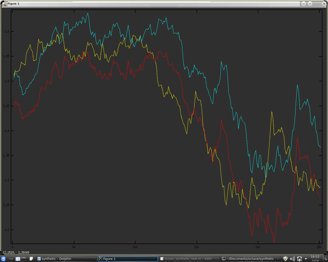
The function produces a permuted time series that preserves the trend of the original time series ( begins and ends with the same values for both the permuted and unpermuted data ) as can be seen in this screen shot of typical output, plotted using Gnuplot,
where the yellow is the real ( in this case S & P 500 ) data and the red and blue bars are a typical example of a single permutation run. This next screen shot shows that part of the above where the two series overlap on the right hand side, so that the details can be visually compared.
The purpose and necessity for this will be explained in a future post, where the planned tests will be discussed in more detail.