Expressing an Indicator in Neural Net Form, Part 3.

The results of the first set of tests of optimising an indicator via the framework of training a neural net are in, and this post is a presentation of these results and a reflection on this in more general terms. I would encourage readers to look at my previous 2 posts to put this one in context.

The following chart plot shows 8 weeks of 10 minute price action in the EURUSD forex pair, with the white equity curve being the cumulative sum of open to open tick returns over this period. The green equity curve is a similar cumulative sum of the tick returns based on going long/short when the basic indicator crosses above/below its zero line. Finally, the mass of magenta coloured equity curves are those that result from various simple moving average smoothing, momentum of and smooths of momentum, and short term MACDs of the basic indicator, with the same zero line crossing positioning.  

These different magenta equity curves are expressed by setting different weights for the "decision weights" shown in the neural net diagram in the previous 2 posts, e.g. a weight matrix [ 0.25 0.25 0.25 0.25 ] is obviously a 4 bar simple moving, whilst weight matrices [ 0.25 0.25 -0.5 -0.5 ] and [ -0.25 -0.25 0.5 0.5 ] are MACDs of 2 bar fast and 4 bar slow simple moving averages (respectively a fast minus slow MACD and slow minus fast MACD - short term trend following vs. mean reversion?) In this way it is possible to create all the various smooths etc. shown above.

Taking this idea a bit further, it is possible to characterise the more "traditional" way of back testing, i.e. testing over a range of possible indicator look back periods, smooths etc. as an extremely limited or constrained form of neural net training. Consider the neural net diagram of my previous posts - a "traditional" back test is functionally equivalent to:-

• setting the neural net architecture as shown in the above mentioned diagram, but only allowing linear hidden activation units
• not allowing the addition of any bias units
• fixing the input weights and output weights matrices prior to any training and not allowing any updating of these weights to take place
• and only allowing the decision weights to be updated, and limiting this updating to a choice between a limited set of fixed weights and not allowing any error based backpropagation to take place

The next chart plot shows the out of sample result of such limited training. The white and green equity curves are the same as previously described, the cumulative sum of open to open returns and zero line crossings of the basic indicator. The single magenta coloured equity curve is the result of following this limited, "traditional" walk forward optimization 

• choose the best set of fixed decision weights over a 2 week window. This best set is decided by choosing the equity curve with the highest Sortino ratio. For the first train/test iteration the 2 week window of training data is not shown but is that data immediately prior to the left hand edge of the plot
• this best set is used out of sample over 1 week of data, the first week of the shown magenta equity curve
• at the end of this first test week, roll the training window forward 1 week so that the new training data consists of the latter week of the first set of training data and the data that has just formed the test week
• repeat the training over this new set of 2 week training data and test out of sample on the immediately following week's data
• keep rolling the window forward, repeating the above, until the end of the test period  

The red equity curve is the equity curve that comes from the decision weights that are equivalent to a 3 bar simple moving average of the 1 bar momentum of the basic indicator, shown because this was visually identified in the first post in this series as being "the best." Comparing this equity curve with the magenta ones in the first chart it is obvious that this set of decision weights, out of sample, turns out to be probably the worst of all sets of weights. This is significant because these weights were the ones that were used to initialize the decision weights prior to neural net training.

Finally, the blue equity curve is the out of sample curve for the trained neural net, trained/tested following the same rolling methodology just described above for the magenta curve. In a hand-wavy way, the improvement in performance from the red to the blue equity curves can be said to show the benefits of optimising an indicator's performance via the framework of neural net training. This then begs the question, what if the neural net was initialised with a better set of decision weights, i.e. those of the magenta curve? This will be the subject of my next post.

More in due course. 

Expressing an Indicator in Neural Net form, Part 2.

Following on from my previous post, I have been experimenting with various tweaks to the basic set-up of expressing an indicator in the form of a neural net, shown again below to avoid the necessity of having readers flip between posts. 

The tweaks explored relate to the weight matrices, activation functions, targets and loss functions, the end results of which are now briefly summarized in turn.

The weight matrices are sparse and with shared weights within each separate matrix because they simply calculate the 4 indicator outputs t which represent the indicator and 3 lagged outputs of it, hence sharing the same weights. The input weights matrix is a 40 by 20 matrix with only 10 unique parameters to train/update (expressed during training by averaging across the 40 non zero weights in the matrix). Similarly, the output weights matrix only has 1 unique trainable weight. Together with bias units (not shown in the diagram above) and the 4 decision weights, the whole neural net has a total of 16 trainable weights.

The activation units are exactly as discussed in my previous post and shown in the diagram above, namely tanh on the 2 hidden layers and a sigmoid on the final output layer.

For the targets I used the sign of the slope of a sliding, centred smooth of the OHLC bar opens, on the premise that the first trade opportunity would be acted upon at the opening price following a buy/sell signal calculated on the close of a bar. The smoothing eliminates the whipsaws that would result from a single adverse return in an otherwise smooth set of returns.   

The loss is a combination of a weighted cross-entropy loss and a Sortino ratio loss. The weights for the weighted cross-entropy loss are simply the absolute values of the returns, the idea being that it is more important to get the direction right on the big returns. The Sortino loss is implemented by minimizing the negative of the Sortino ratio, i.e. maximizing the ratio. There are 2 versions of this Sortino loss: an analytical gradient that spreads the cost over each training sample per training epoch similar to the cross-entropy loss, and a global loss which uses finite differences over the 4 output decision weights. Both of these Sortino losses were coded with the help of deepseek-talkai. The losses are mixed via a mixing parameter, Lambda, which varies from 0 to 1, with 0 being a pure cross-entropy loss and 1 being pure Sortino loss. 

The following .gif shows the training data equity curves for each type of loss (see the titles of each plot) for every hundredth epoch up to epoch 600 over a week's worth of 10 minute forex data limited to the trading hours described in my previous post. The legend in the top left corner identifies each equity curve.

Obviously these plots show that it is possible to improve results over those of the original indicator (shown in red in the above .gif), but of course these are in-sample results. My next post will be about cross validation and out-of sample test results.
 

Expressing an Indicator in Neural Net Form

Recently I started investigating relative rotation graphs with a view to perhaps implementing a version of this for use on forex currency pairs. The underlying idea of a relative rotation graph is to plot an asset's relative strength compared to a benchmark and the momentum of this relative strength and to plot this in a form similar to a Polar coordinate system plot, which rotates around a zero point representing zero relative strength and zero relative strength momentum. After some thought it occurred to me that rather than using relative strength against a benchmark I could use the underlying relative strengths of the individual currencies, as calculated by my currency strength indicator, against each other. Furthermore, these underlying log changes in the individual currencies can be normalised using the ideas of brownian motion and then averaged together over different look back periods to create a unique indicator.

This indicator was coded up in the "traditional" way that will be familiar to anybody who has ever tried coding a trading indicator in any coding language. However, I thought that if the calculation of this indicator could be expressed in the form of a Feedforward neural network then the optimisation opportunities available using backpropagation and regularization could be used to tweek the indicator in more useful ways than just varying a look back length and amount of averaging. After some work I was able to make this work in just these two lines of Octave code:

indicator_middle_layer = tanh( full_feature_matrix * input_weights ) ;
indicator_nn_output = tanh( indicator_middle_layer * output_weights ) ; 

Of course, prior to calling these two lines of code, there is some feature engineering to create the input full_feature_matrix, and the input weights and output_weights matrices taken together are mathematically equivalent to the original indicator calculations. Finally, because this is a neural net expression of the indicator, the non-linear tanh activation function is applied to the hidden middle and output layers of the net.

The following plot shows the original indicator in black and the neural net version of it in blue 

over the data shown in this plot of 10 minute bars of the EURUSD forex pair. 

The red indicator in the plot above is the 1 bar momentum of the neural net indicator plot.

To judge the quality of this indicator I used the entropy measure (measured over 14,000+ 10 minute bars of EURUSD), the results of which are shown next.

entropy_indicator_original = 0.9485
entropy_indicator_nn_output = 0.9933

An entropy reading of 0.9933 is probably as good as any trading indicator could hope to achieve (a perfect reading is 1.0) and so the next thing was to quickly back test the indicator performance. Based on the logic of the indicator the obvious long (short) signals are being above (below) the zeroline, or equivalently the sign of the indicator, and for good measure I also tested the sign of the momentum and some simple moving averages thereof.

The following plot shows the equity curves of this quick test where it is visually clear that the blue equity curves are "the best" when plotted in relation to the black "buy and hold" equivalent equity curve. These represent the equity curves of a 3 bar simple moving average of the 1 bar momentum of both the original formulation of the indicator and the neural net implementation. I would point out that these equity curves represent the theoretical equity resulting from trading the London session after 9:00am BST and stopping at 7:00am EST (usually about noon BST) and then starting trading again at 9:00am EST until 17:00pm EST. This schedule avoids the opening sessions (7:00 to 9:00am) in both London and New York because, from my observations of many OHLC charts such as shown above, there are frequently wild swings where price is being pushed to significant points such as volume profile clusters, accumulations of buy/sell orders etc. and in my opinion no indicator can be expected to perform well in that sort of environment. Also avoided are the hours prior to 7:00am BST, i.e. the Asian session or overnight session.    

Although these equity curves might not, at first glance, be that impressive, especially as they do not account for trading costs etc. my intent on doing these tests was to determine the configuration of a final "decision" output layer to be added to the neural net implementation of the indicator. A 3 bar simple moving average of the 1 bar momentum implies the necessity to include 4 consecutive readings of the indicator output as input to a final " decision" layer. The following simple, hand-drawn sketch shows what I mean:

A discussion of this will be the subject of my next post.

Indicator(s) Derived from PositionBook Data

Since my last post I have been trying to create new indicators from PositionBook data but unfortunately I have had no luck in doing so. I have have tried differences, ratios, cumulative sums, logs and control charts to no avail and I have decided to discontinue this line of investigation because it doesn't seem to hold much promise. The only other direct uses I can think of for this data are:

• modifying existing indicators that use volume such as Accumulation/distribution index, On balance volume and Money flow index. The idea would be to use the PositionBook data relationships instead of the price bar relationships to calculate the intermediate steps of CLV and Money Ratio.
• create a sort of PositionBook profile chart, similar to a volume profile chart. However, I suspect that this would be redundant as the high/low PositionBook nodes would be almost identical to the high/low volume nodes.
• directly use the PositionBook data as input to a machine learning model, either as a stand alone "indicator" or in a Meta learning paradigm as outlined in Advances in Financial Machine Learning.

I am not yet sure which of the above I will look at next, but whichever it is will be the subject of a future post.

Simple Machine Learning Models on OrderBook/PositionBook Features

This post is about using OrderBook/PositionBook features as input to simple machine learning models after previous investigation into the relevance of such features. 

Due to the amount of training data available I decided to look only at a linear model and small neural networks (NN) with a single hidden layer with up to 6 hidden neurons. This choice was motivated by an academic paper I read online about linear models which stated that, as a lower bound, one should have at least 10 training examples for each parameter to be estimated. Other online reading about order flow imbalance (OFI) suggested there is a linear relationship between OFI and price movement. Use of limited size NNs would allow a small amount of non linearity in the relationship. For this investigation I used the Netlab toolbox and Octave. A plot of the learning curves of the classification models tested is shown below. The targets were binary 1/0 for price increases/decreases.

The blue lines show the average training error (y axis) and the red lines show the same average error metric on the held out cross validation data set for each tested model. The thickness of the lines represents the number of neurons in the single hidden layer of the NNs (the thicker the lines, the higher the number of hidden neurons). The horizontal green line shows the error of a generalized linear model (GLM) trained using iteratively reweighted least squares. It can be seen that NN models with 1 and 2 hidden neurons slightly outperform the GLM, with the 2 neuron model having the edge over the 1 neuron model. NN models with 3 or more hidden neurons over fit and underperform the GLM. The NN models were trained using Netlab's functions for Bayesian regularization over the parameters.

Looking at these results it would seem that a 2 neuron NN would be the best choice; however the error differences between the 1 and 2 neuron NNs and GLM are small enough to anticipate that the final classifications (with a basic greater/less than a 0.5 logistic threshold value for long/short) would perhaps be almost identical. 

Investigations into this will be the subject of my next post. 

The code box below gives the working Octave code for the above.

## load data
##training_data = dlmread( 'raw_netlab_training_features' ) ;
##cv_data = dlmread( 'raw_netlab_cv_features' ) ;
training_data = dlmread( 'netlab_training_features_svd' ) ;
cv_data = dlmread( 'netlab_cv_features_svd' ) ;
training_targets = dlmread( 'netlab_training_targets' ) ;
cv_targets = dlmread( 'netlab_cv_targets' ) ;

kk_loop_record = zeros( 30 , 7 ) ;

for kk = 1 : 30
  
## first train a glm model as a base comparison
input_dim = size( training_data , 2 ) ; ## Number of inputs.

net_lin = glm( input_dim , 1 , 'logistic' ) ; ## Create a generalized linear model structure.
options = foptions ; ## Sets default parameters for optimisation routines, for compatibility with MATLAB's foptions()
options(1) = 1 ;  ## change default value
##	OPTIONS(1) is set to 1 to display error values during training. If
##	OPTIONS(1) is set to 0, then only warning messages are displayed.  If
##	OPTIONS(1) is -1, then nothing is displayed.
options(14) = 5 ; ## change default value
##	OPTIONS(14) is the maximum number of iterations for the IRLS
##	algorithm;  default 100.
net_lin = glmtrain( net_lin , options , training_data , training_targets ) ;

## test on cv_data
glm_out = glmfwd( net_lin , cv_data ) ;
## cross-entrophy loss
glm_out_loss = -mean( cv_targets .* log( glm_out )  .+ ( 1 .- cv_targets ) .* log( 1 .- glm_out ) ) ;

kk_loop_record( kk , 7 ) = glm_out_loss ;

## now train an mlp
## Set up vector of options for the optimiser.
nouter = 30 ; ## Number of outer loops.
ninner = 2 ;	## Number of innter loops.
options = foptions ; ## Default options vector.
options( 1 ) = 1 ;	## This provides display of error values.
options( 2 ) = 1.0e-5 ; ## Absolute precision for weights.
options( 3 ) = 1.0e-5 ; ## Precision for objective function.
options( 14 ) = 100 ; ## Number of training cycles in inner loop.

training_learning_curve = zeros( nouter , 6 ) ; 
cv_learning_curve = zeros( nouter , 6 ) ;

for jj = 1 : 6

## Set up network parameters.
nin = size( training_data , 2 ) ; ## Number of inputs.
nhidden = jj ;	## Number of hidden units.
nout = 1 ; ## Number of outputs.
alpha = 0.01 ; ## Initial prior hyperparameter.
aw1 = 0.01 ;
ab1 = 0.01 ;
aw2 = 0.01 ;
ab2 = 0.01 ;

## Create and initialize network weight vector.
prior = mlpprior(nin , nhidden , nout , aw1 , ab1 , aw2 , ab2 ) ;
net = mlp( nin , nhidden , nout , 'logistic' , prior ) ;

## Train using scaled conjugate gradients, re-estimating alpha and beta.
for ii = 1 : nouter
  ## train net
  net = netopt( net , options , training_data , training_targets , 'scg' ) ;
  
  train_out = mlpfwd( net , training_data ) ;
  ## get train error
  ## mse
  ##training_learning_curve( ii ) = mean( ( training_targets .- train_out ).^2 ) ;
  
  ## cross entropy loss
  training_learning_curve( ii , jj ) = -mean( training_targets .* log( train_out )  .+ ( 1 .- training_targets ) .* log( 1 .- train_out ) ) ; 

  cv_out = mlpfwd( net , cv_data ) ;
  ## get cv error
  ## mse
  ##cv_learning_curve( ii ) = mean( ( cv_targets .- cv_out ).^2 ) ;
  
  ## cross entropy loss
  cv_learning_curve( ii , jj ) = -mean( cv_targets .* log( cv_out )  .+ ( 1 .- cv_targets ) .* log( 1 .- cv_out ) ) ; 
  
  ## now update hyperparameters based on evidence
  [ net , gamma ] = evidence( net , training_data , training_targets , ninner ) ;
  
##  fprintf( 1 , '\nRe-estimation cycle ##d:\n' , ii ) ;
##  disp( [ '  alpha = ' , num2str( net.alpha' ) ] ) ;
##  fprintf( 1 , '  gamma =  %8.5f\n\n' , gamma ) ;
##  disp(' ')
##  disp('Press any key to continue.')
  ##pause;
endfor ## ii loop

endfor ## jj loop

kk_loop_record( kk , 1 : 6 ) = cv_learning_curve( end , : ) ;

endfor ## kk loop

plot( training_learning_curve(:,1) , 'b' , 'linewidth' , 1 , cv_learning_curve(:,1) , 'r' , 'linewidth' , 1 , ...
training_learning_curve(:,2) , 'b' , 'linewidth' , 2 , cv_learning_curve(:,2) , 'r' , 'linewidth' , 2 , ...
training_learning_curve(:,3) , 'b' , 'linewidth' , 3 , cv_learning_curve(:,3) , 'r' , 'linewidth' , 3 , ...
training_learning_curve(:,4) , 'b' , 'linewidth' , 4 , cv_learning_curve(:,4) , 'r' , 'linewidth' , 4 , ...
training_learning_curve(:,5) , 'b' , 'linewidth' , 5 , cv_learning_curve(:,5) , 'r' , 'linewidth' , 5 , ...
training_learning_curve(:,6) , 'b' , 'linewidth' , 6 , cv_learning_curve(:,6) , 'r' , 'linewidth' , 6 , ...
ones( size( training_learning_curve , 1 ) , 1 ).*glm_out_loss , 'g' , 'linewidth', 2 ) ;

##  >> mean(kk_loop_record)
##  ans =
##
##     0.6928   0.6927   0.7261   0.7509   0.7821   0.8112   0.6990

##  >> std(kk_loop_record)
##  ans =
##
##     8.5241e-06   7.2869e-06   1.2999e-02   1.5285e-02   2.5769e-02   2.6844e-02   2.2584e-16

OrderBook and PositionBook Features

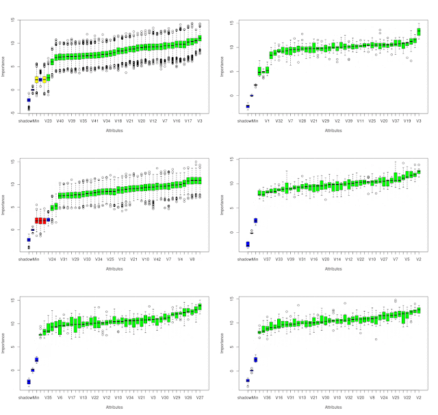
In my previous post I talked about how I planned to use constrained optimization to create features from Oanda's OrderBook and PositionBook data, which can be downloaded via their API. In addition to this I have also created a set of features based on the idea of Order Flow Imbalance (OFI), a nice exposition of which is given in this blog post along with a numerical example of how to calculate OFI. Of course Oanda's OrderBook/PositionBook data is not exactly the same as a conventional limit order book, but I thought they are similar enough to investigate using OFI on them. The result of these investigations is shown in the animated GIF below.

This shows the output from using the R Boruta package to check for the feature relevance of OFI levels to a depth of 20 of both the OrderBook and PositionBook to classify the sign of the log return of price over the periods detailed below following an OrderBook/PositionBook update (the granularity at which the OrderBook/PositionBook data can be updated is 20 minutes):

• 20 minutes
• 40 minutes
• 60 minutes
• the 20 minutes starting 20 minutes in the future
• the 20 minutes starting 40 minutes in the future

for both the OrderBook and PositionBook, giving a total of 10 separate images/results in the above GIF.

 

Observant readers may notice that in the GIF there are 42 features being checked, but only an OFI depth of 20. The reason for this is that the data contain information about buys/sell orders and long/short positions both above and below the current price, so what I did was calculate OFI for:

• buy orders above price vs sell orders below price
• sell orders above price vs buy orders below price
• long positions above price vs short positions below price
• short positions above price vs long positions below price 

As can be seen, almost all features are deemed to be relevant with the exception of 3 OFI levels rejected (red candles) and 2 deemed tentative (yellow candles).

It is my intention to use these features in a machine learning model to classify the probability of future market direction over the time frames mentioned above. 

More in due course.

Time Warp Edit Distance as a Loss Function

Some time ago I posted about the time warp edit distance (twed) and recently I've revisited this as a possible loss function. The basic idea is to use this during algorithm training to match a "perfect equity curve" rather than use the usual loss measurements such as mean squared error for regression or cross entropy for classification.

As a proof of concept I've been playing around with this Octave script

clear all ;
1 ;

function J = twed_loss( x )
 global price ;
 global returns ;
 global perfect_equity_curve ; 
 fast_ma = sma( price , round( x( 1 ) ) ) ;
 slow_ma = sma( price , round( x( 2 ) ) ) ;
 test_position_vector = sign( fast_ma .- slow_ma ) ;
 test_position_vector = shift( test_position_vector , 2 ) ;
 test_position_vector( 1 : 3 ) = 0 ;
 test_equity_curve = cumsum( returns .* test_position_vector ) ;
 x_axis = ( 1 : numel( perfect_equity_curve ) )' ;
 J = twed( perfect_equity_curve , x_axis , test_equity_curve , x_axis , 1 , 0.001 ) ;
endfunction

## create a perfectly predictable price
global price = sinewave( 200 , 20 )' .+ 5 ;
global returns = [ 0 ; diff( price ) ] ;
perfect_position_vector = sign( returns ) ;
perfect_position_vector = shift( perfect_position_vector , 2 ) ; 
perfect_position_vector( 1 : 3 ) = 0 ;
global perfect_equity_curve = cumsum( returns .* perfect_position_vector ) ;

## now do the Baysian training
## set up the parameters for bayesopt
params.n_iterations = 300 ; ## 190
params.n_init_samples = 10 ; ## 10
params.n_iter_relearn = 1 ; ## Number of iterations between re-learning kernel parameters. That is, kernel learning ocur 1 out of n_iter_relearn iterations. 
## Ideally, the best precision is obtained when the kernel parameters are learned every iteration (n_iter_relearn=1). 
## However, this learning part is computationally expensive and implies a higher cost per iteration. If n_iter_relearn=0, then there is no relearning. [Default 50]
params.crit_name = 'cEI' ;
params.surr_name = 'sStudentTProcessNIG' ;
params.noise = 1e-6 ;
params.kernel_name = 'kMaternARD5' ;
params.kernel_hp_mean = [ 1 ] ;
params.kernel_hp_std = [ 10 ] ;
params.verbose_level = 0 ; ## Negative -> Error -> stdout 0 -> Warning -> stdout 1 -> Info -> stdout 2 -> Debug -> stdout
                           ## 3 -> Warning -> log file 4 -> Info -> log file 5 -> Debug -> log file 5 -> Error -> log file
params.load_save_flag = 0 ; ## 1-Load data, 2-Save data, 3-Load and append data. Other values, no file saving or restore [Default 0]
params.log_filename = '/home/dekalog/Documents/octave/twed/bayeopt.log' ; % Name/path of the log file 
## (if applicable, verbose_level>=3) [Default "bayesopt.log"]
params.load_filename = '/home/dekalog/Documents/octave/twed/bayeopt.log' ;
params.save_filename = '/home/dekalog/Documents/octave/twed/bayeopt.log' ;

lb = [ 2 3 ] ;
## upper bounds
ub = [ 30 30 ] ;
nDimensions = length( lb ) ;
[ xmin , fmin ] = bayesoptcont( 'twed_loss' , nDimensions , params , lb , ub ) ;
round( xmin )
fmin

fast_ma = sma( price , round( xmin(1) ) ) ;
slow_ma = sma( price , round( xmin(2) ) ) ;
figure(1) ; plot(price,'k','linewidth',2,fast_ma,'r','linewidth',2,slow_ma,'b','linewidth',2 ) ;
title( 'PRICE AND MA CROSSOVER SIGNALS' ) ; legend( 'PRICE' , 'FAST MA' , 'SLOW MA' ) ;
test_position_vector = sign( fast_ma .- slow_ma ) ;
test_position_vector = shift( test_position_vector , 2 ) ;
test_position_vector( 1 : 3 ) = 0 ;
test_equity_curve = cumsum( returns .* test_position_vector ) ; 
figure(2) ; plot(perfect_equity_curve,'b','linewidth',2,test_equity_curve,'r','linewidth',2) ;
title( 'EQUITY CURVES' ) ; legend( 'PERFECT EQUITY CURVE' , 'TEST EQUITY CURVE' ) ;

which produces plots such as this

and this,

which both show a fast and slow moving average crossover system on sine wave "price" of period 20, optimised to match equity curves such as below via the twed loss.

What is interesting about this is that the moving average lengths usually converge to more or less the expected theoretical optimum, with the required change of sign of signal, where the crossovers indicate peaks and troughs in price and hence perfect entry and exit signals.

However, sometimes the solution looks like this,

which is an 11 period fast moving average and a 10 period slow one, quite a contrarian solution compared to the theoretical optimum, but actually giving a lower twed loss.

I quite like the idea of optimising for what we actually care about, i.e. the equity curve, whilst at the same time possibly uncovering unique solutions. It seems that the twed loss shows promise.

More in due course.

More Work on RVFL Networks

Back in November last year I posted about Random Vector Functional Link (RVFL) networks here and here. Since then, along with my recent work on Oanda's API Octave functions and Market/Volume Profile visualisation, I have continued looking at RVFL networks and this post is an update on this work.

The "random" in RVFL means random initialisation of weights that are then fixed. It seems to me that it might be possible to do better than random by having some principled way of weight initialisation. To this end I have used the Penalised MATLAB Toolbox on features derived from my ideal cyclic tau embedding function to at first train a Generalized Linear Model with the Lasso penalty and then the Ridge penalty over thousands of sets of Monte Carlo generated, ideal cyclic prices and such prices with trends. The best weights for each set of prices were recorded in an array and then the mean weight (and standard deviation) taken. This set of mean weights is intended to replace the random weights in a RVFL network designed to predict the probability of "price" being at a cyclic turning point using the above cyclic tau embedding features.

Of course these weights could be considered a trained model in and of themselves, and the following screenshots show "out of sample" performance on Monte Carlo generated ideal prices that were not used in the training of the mean weights.

The black line is the underlying cyclic price and the red, blue and green lines are the mean weight model probabilities for cyclic peaks, troughs or neither respectively. Points where the peak/trough probabilities exceed the neither probabilities are marked by the red and blue vertical lines. Similarly, we have prices trending up in a cyclic fashion

and also trending down

In the cases of the last two trending markets only the swing highs and lows are indicated. The reason for this is that during training, based on my "expert knowledge" of the cyclic tau features used, it is unreasonable to expect these features to accurately capture the end of an up leg in a bull trend or the end of a down leg in a bear trend - hence these were not presented as a positive class during training.

As I said above the motivation for this is to get a more meaningful hidden layer in a RVFL network. This hidden layer will consist of seven Sigmoid functions which each give a probability of price being at or not being at a cyclic turn, conditional upon the type of market the input weights were trained on.

More in due course.

Preliminary Results from Weight Agnostic Training

Following on from my last post, below is a selection of the typical resultant output from the Bayesopt Library minimisation

    3    3    2    2    2    8   99   22   30    1
    3    3    2    3    2   39    9   25   25    1
    2    2    3    2    2   60   43   83   54    3
    2    1    2    2    2    2    0   90   96   43
    3    2    3    2    2    2    2   43   33    1
    2    3    2    3    2    2    0   62   98   21
    2    2    2    2    2   18   43   49    2    2
    2    3    2    4    1    2    0   23    0    0
    2    2    1    2    3    2    0   24   63   65
    3    2    2    2    3    5   92   49    1    0
    2    3    2    1    1    7   84   22   17    1
    3    2    4    1    1   46    1    0   99    7
    2    2    3    2    2    2    0   74   82   50
    3    3    2    2    2   45   14   81   23    2
    2    3    3    2    2    2    0   99   79    4
    2    2    2    2    2    2    0    0   68    0
    3    3    3    2    2   67   17   37   84    1
    3    2    3    2    2   24   39   56   55    1
    3    3    4    3    2    2   30   62   67    1
    2    2    2    2    2    2    1    0    4    0
    2    2    2    2    2    2    9    8   45    1
    2    3    3    2    2   48    1   18   28    1
    2    3    3    2    2    2    0   34   42   18
    2    2    2    3    2    2    0   70   81   10
    2    2    3    3    2    2    0   85   23   11

where the rows are separate run's results, the first five columns show the type of activation function per layer and the last five columns show the number of neurons per layer ( see function code in my last post for details. )

Some quick take aways from this are:

1. the sigmoid activation function ( bounded 0 to 1 ) is not favoured, with either the Tanh or "Lecun" sigmoid ( see section 4.4 of this paper ) being preferred
2. 40% of the network architectures are single hidden layer with just 2 neurons in the hidden layer 
3. 8% have only two hidden layers with the second hidden layer having just one neuron

I would say these preliminary results suggest that a deep architecture is not necessary for the features/targets being tested and obviously the standard sigmoid/logistic function should be avoided.

As is my wont whilst waiting for lengthy computer tests to complete I have also been browsing online, motivated by the early results of the above, and discovered Random Vector Functional Link Networks, which seem to be a precursor to Extreme Learning Machines. However, there appears to be some controversy about whether or not Extreme Learning Machines are just plagiarism of earlier ideas, such as RVFL networks. 

Readers may remember that I have used ELMs before with the Bayesopt library ( see my post here ) and now that the above results point towards the use of shallow networks I intend to replicate the above, but using RVFL networks. This will be the subject of my next post.   

Weight Agnostic Neural Net Training

I have recently come across the idea of weight agnostic neural net training and have implemented a crude version of this combined with the recent work I have been doing on Taken's Theorem ( see my posts here, here and here ) and using the statistical mechanics approach to creating synthetic data.

Using the simple Octave function below with the Akaike Information Criterion as the minimisation objective

## Copyright (C) 2019 dekalog
## 
## This program is free software: you can redistribute it and/or modify it
## under the terms of the GNU General Public License as published by
## the Free Software Foundation, either version 3 of the License, or
## (at your option) any later version.
## 
## This program is distributed in the hope that it will be useful, but
## WITHOUT ANY WARRANTY; without even the implied warranty of
## MERCHANTABILITY or FITNESS FOR A PARTICULAR PURPOSE.  See the
## GNU General Public License for more details.
## 
## You should have received a copy of the GNU General Public License
## along with this program.  If not, see
## .

## -*- texinfo -*- 
## @deftypefn {} {@var{J} =} wann_training_of_cyclic_embedding()
##
## @seealso{}
## @end deftypefn

## Author: dekalog 
## Created: 2019-10-26

function J = wann_training_of_cyclic_embedding( x )
global sample_features ; global sample_targets ;
epsilon = 1e-15 ; ## to ensure log() does not give out a nan

## get the parameters from input x
activation_funcs = floor( x( 1 : 5 ) ) ; ## get the activations, 1 == sigmoid, 2 == tanh, 3 == Lecun sigmoid
layer_size = floor( x( 6 : 10 ) ) ;

[ min_layer_size , ix_min ] = min( layer_size ) ;
  if( min_layer_size > 0 ) ## to be expected most of the time
    nn_depth = length( layer_size ) ;
  elseif( min_layer_size == 0 ) ## one layer has no nodes, hence limits depth of nn
    nn_depth = ix_min - 1 ;
  endif 

length_jj_loop = 25 ;
all_aic_values = zeros( length_jj_loop , 1 ) ;  
  
for jj = 1 : length_jj_loop 
  
  previous_layer_out = sample_features ;
  sum_of_k = 0 ;
    
  for ii = 1 : nn_depth
    
    new_weight_matrix = ones( size( previous_layer_out , 2 ) , layer_size( ii ) ) ./ sqrt( size( previous_layer_out , 2 ) ) ;
    sum_of_k = sum_of_k + numel( new_weight_matrix ) ;
    prior_to_activation_input = previous_layer_out * new_weight_matrix ;

    ## select the activation function 
    if( activation_funcs( ii ) == 1 ) ## sigmoid activation
      previous_layer_out = 1.0 ./ ( 1.0 .+ exp( -prior_to_activation_input ) ) ;
    elseif( activation_funcs( ii ) == 2 ) ## tanh activation
      previous_layer_out = tanh( prior_to_activation_input ) ;
    elseif( activation_funcs( ii ) == 3 ) ## lecun sigmoid activation
      previous_layer_out = sigmoid_lecun_m( prior_to_activation_input ) ;
    endif 
    
  endfor

  ## the final logistic output
  new_weight_matrix = ones( size( previous_layer_out , 2 ) , 1 ) ./ sqrt( size( previous_layer_out , 2 ) ) ;
  sum_of_k = sum_of_k + numel( new_weight_matrix ) ;
  final_output = previous_layer_out * new_weight_matrix ;
  final_output = 1.0 ./ ( 1.0 .+ exp( -final_output ) ) ;

  max_likelihood = sum( log( final_output .+ epsilon ) .* sample_targets + log( 1 .- final_output .+ epsilon ) .* ( 1 .- sample_targets ) ) ;
  
  ## get Akaike Information criteria
  all_aic_values( jj ) = 2 * sum_of_k - 2 * max_likelihood ;

endfor ## end of jj loop

J = mean( all_aic_values ) ;

endfunction

and the Octave interface of the Bayesopt Library I am currently iterating over different architectures ( up to 5 hidden layers deep with a max of 100 nodes per layer and using a choice of 3 hidden activations ) for a simple Logistic Regression model to predict turning points in different sets of statistical mechanics synthetic data using just features based on Taken's embedding.

More in due course.

Ideal Cyclic Tau Embedding as Times Series Features

Continuing on from my Ideal Tau for Time Series Embedding post, I have now written an Octave function based on these ideas to produce features for time series modelling. The function outputs are two slightly different versions of features, examples of which are shown in the following two plots, which show up and down trends in black, following a sinusoidal sideways market partially visible to the left:

and

The function outputs are normalised price and price delayed by a quarter and a half of the cycle period (in this case 20.) The trend slopes have been chosen to exemplify the difference in the features between up and down trends. The function outputs are identical for the unseen cyclic prices to the left.

When the sets of function outputs are plotted as 3D phase space plots typical results are

with the green, blue and red phase trajectories corresponding to the cyclic, up trending and down trending portions of the above synthetic price series. The markers in this plot correspond to points in the phase trajectories at which turns in the underlying price series occur. The following plot is the above plot rotated in phase space such that the green cyclic price phase trajectory is horizontally orientated.

It is clearer in this second phase space plot that there is a qualitative difference in the phase space trajectories of the different, underlying market types.

As a final check of feature relevance I used the Boruta R package, with the above turning point markers as classification targets (a turning point vs. not a turning point,) to assess the utility of this approach in general. These tests were conducted on real price series and also on indices created by my currency strength methodology. In all such Boruta tests the features are deemed "relevant" up to a delay of five bars on daily data (I ceased the tests at the five bar mark because it was becoming tedious to carry on.)

In summary, therefore, it can be concluded that features derived using Taken's theorem are useful on financial time series provided that:

1. the underlying time series are normalised (detrended) and,
2. the embedding delay (Tau) is set to the theoretical optimum of a quarter (and multiples thereof) of the measured cyclic period of the time series.

"Black Swan" Data Cleaning

Since my last post I have been investigating training features that can be derived from my Currency Strength indicator as input for machine learning algorithms and during this work it was obvious that there are instances in the raw data that are Black Swan outliers. This can be seen in the chart below as pronounced spikes.

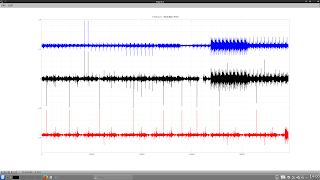
The chart itself is a plot of log returns of various forex crosses and Gold and Silver log returns, concatenated into one long vector. The black is the actual return of the underlying, the blue is the return of the base currency and the red is the cross currency, both of these being calculated from indices formed from the currency strength indicator.

By looking at the dates these spikes occur and then checking online I have flagged four historical "Black swan" events that occured within the time frame the data covers, which are listed in chronological order below:

1. Precious metals price collapse in mid April 2013
2. Swiss Franc coming off its peg to the Euro in January 2015
3. Fears over the Hong Kong dollar and Renminbi currency peg in January 2016
4. Brexit black Friday

The next series of charts shows the progressive reduction in the number of spikes as the data around the above events is deleted from those crosses etc. that were affected.

It can be seen that the final chart shows much more homogeneous data within each concatenated series, which should have benefits when said data is used as machine learning input. Also, the data that has been deleted will provide a useful, extreme test set to stress test any finished model. More in due course.

Update on Currency Strength Smoothing, and a new direction?

Since my last two posts ( currency strength indicator and preliminary tests thereof ) I have been experimenting with different ways of smoothing the indicators without introducing lag, mostly along the lines of using an oscillator leading signal plus various schemes to smooth and compensate for introduced attenuation and making heavy use of my particle swarm optimisation code. Unfortunately I haven't found anything that really works to my satisfaction and so I have decided to forgo any further attempts at this and just use the indicator in its unsmoothed form as neural net input.

In the process of doing the above work I decided that my particle swarm routine wasn't fast enough and I started using the BayesOpt optimisation library, which is written in C++ and has an interface to Octave. Doing this has greatly decreased the time I've had to spend in my various optimisation routines and the framework provided by the BayesOpt library will enable more ambitious optimisations in the future.

Another discovery for me was this Predicting Stock Market Prices with Physical Laws paper, which has some really useful ideas for neural net input features. In particular I think the idea of combining position, velocity and acceleration with the ideas contained in an earlier post of mine on Savitzky Golay filter convolution and using the currency strength indicators as proxies for the arbitrary sine and cosine waves function posited in the paper hold some promise. More in due course.    

Possible Addition of NARX Network to Conditional Restricted Boltzmann Machine

It has been over three months since my last post, due to working away from home for some of the summer, a summer holiday and moving home. However, during this time I have continued with my online reading and some new thinking about my conditional restricted boltzmann machine based trading system has developed, namely the use of a nonlinear autoregressive exogenous model in the bottom layer gaussian units of the CRBM. Some links to reading on the same are shown below.

• https://www.mathworks.com/help/nnet/ug/design-time-series-narx-feedback-neural-networks.html 
• http://deeplearning.cs.cmu.edu/pdfs/Narx.pdf 
• http://www.wseas.us/e-library/transactions/research/2008/27-464.pdf 
• https://rucore.libraries.rutgers.edu/rutgers-lib/24889/ 
• https://arxiv.org/abs/1607.02093 
• https://hal.archives-ouvertes.fr/hal-00501643/document 
• http://www.theijes.com/papers/v3-i11/Version-1/C0311019026.pdf 
• http://www.sciencedirect.com/science/article/pii/S0925231208003081 

The exogenous time series I am thinking of using, at least for the major forex pairs and perhaps precious metals, oil and US treasuries, is a currency strength indicator based on the US dollar. In order to create the currency strength indicator I will have to delve into some data wrangling with the historical forex data I have, and this will be the subject of my next post.

Parallel Tempering and Adaptive Learning Rates in Restricted Boltzmann Machine Learning

It has been a while since my last post and in the intervening time I have been busy working on the code of my previous few posts.

During the course of this I have noticed that there are some further improvements to be made in terms of robustness etc. inspired by this Master's thesis, Improved Learning Algorithms for Restricted Boltzmann Machines, by KyungHyun Cho. Using the Deepmat Toolbox code available here as a guide, I now intend to further improve my code by incorporating the concepts of Parallel Tempering and adaptive learning rates for both the RBM and CRBM training.

More in due course.

Refactored Denoising Autoencoder Update #2

Below is this second code update.

%  select rolling window length to use - an optimisable parameter via pso?
rolling_window_length = 50 ;
batchsize = 5 ;

%  how-many timesteps do we look back for directed connections - this is what we call the "order" of the model 
n1 = 3 ; % first "gaussian" layer order, a best guess just for batchdata creation purposes
n2 = 3 ; % second "binary" layer order, a best guess just for batchdata creation purposes

%  taking into account rolling_window_length, n1, n2 and batchsize, get total lookback length
remainder = rem( ( rolling_window_length + n1 + n2 ) , batchsize ) ;

if ( remainder > 0 ) % number of training examples with lookback and orders n1 and n2 not exactly divisable by batchsize
lookback_length = ( rolling_window_length + n1 + n2 + ( batchsize - remainder ) ) ; % increase the lookback_length
else                 % number of training examples with lookback and orders n1 and n2 exactly divisable by batchsize
lookback_length = ( rolling_window_length + n1 + n2 ) ;
end

%  create batchdataindex using lookback_length to index bars in the features matrix
batchdataindex = ( ( training_point_index - ( lookback_length - 1 ) ) : 1 : training_point_index )' ;
batchdata = features( batchdataindex , : ) ;

%  now that the batchdata has been created, check it for autocorrelation in the features
all_ar_coeff = zeros( size( batchdata , 2 ) , 1 ) ;

  for ii = 1 : size( batchdata , 2 )
  ar_coeffs = arburg( batchdata( : , ii ) , 10 , 'FPE' ) ;
  all_ar_coeff( ii ) = length( ar_coeffs ) - 1 ;
  end
  
%  set order of gaussian_crbm, n1, to be equal to the average length of any autocorrelation in the data
n1 = round( mean( all_ar_coeff ) ) ;  

%  z-normalise the batchdata matrix with the mean and std of columns 
data_mean = mean( batchdata , 1 ) ;
data_std = std( batchdata , 1 ) ;
batchdata = ( batchdata .- repmat( data_mean , size( batchdata , 1 ) , 1 ) ) ./ repmat( data_std , size( batchdata , 1 ) , 1 ) ; % batchdata is now z-normalised by data_mean & data_std

%  create the minibatch index matrix for gaussian rbm pre-training of directed weights w
minibatch = ( 1 : 1 : size( batchdata , 1 ) ) ; minibatch( 1 : ( size( batchdata , 1 ) - rolling_window_length ) ) = [] ;
minibatch = minibatch( randperm( size( minibatch , 2 ) ) ) ; minibatch = reshape( minibatch , batchsize , size( minibatch , 2 ) / batchsize ) ; 

% PRE-TRAINING FOR THE VISABLE TO HIDDEN AND THE VISIBLE TO VISIBLE WEIGHTS %%%%
% First create a training set and target set for the pre-training of gaussian layer
dAuto_Encode_targets = batchdata ; dAuto_Encode_training_data = [] ;
% dAuto_Encode_targets = batchdata( : , 2 : end ) ; dAuto_Encode_training_data = [] ; % if bias added to raw data
  
  % loop to create the dAuto_Encode_training_data ( n1 == "order" of the gaussian layer of crbm )
  for ii = 1 : n1
  dAuto_Encode_training_data = [ dAuto_Encode_training_data shift( batchdata , ii ) ] ;
  end

% now delete the first n1 rows due to circular shift induced mismatch of data and targets
dAuto_Encode_targets( 1 : n1 , : ) = [] ; dAuto_Encode_training_data( 1 : n1 , : ) = [] ;

% DO RBM PRE-TRAINING FOR THE BOTTOM UP DIRECTED WEIGHTS W %%%%%%%%%%%%%%%%%%%%%
% use rbm trained initial weights instead of using random initialisation for weights
% Doing this because we are not using regularisation in the autoencoder pre-training
epochs = 10000 ;
hidden_layer_size = 4 * size( dAuto_Encode_targets , 2 ) ;
[ w_weights , w_weights_hid_bias , w_weights_vis_bias ] = cc_gaussian_rbm( dAuto_Encode_targets , minibatch , epochs , hidden_layer_size , 0.05 ) ;
% keep a copy of these original w_weights
w1 = w_weights ;
[ A_weights , A_weights_hid_bias , A_weights_vis_bias ] = cc_gaussian_rbm( dAuto_Encode_training_data , minibatch , epochs , size( dAuto_Encode_targets , 2 ) , 0.05 ) ;
[ B_weights , B_weights_hid_bias , B_weights_vis_bias ] = cc_gaussian_rbm( dAuto_Encode_training_data , minibatch , epochs , hidden_layer_size , 0.05 ) ;

% END OF RBM PRE-TRAINING OF AUTOENCODER WEIGHTS %%%%%%%%%%%%%%%%%%%%%%%%%%%%%%%

figure(1) ; surf( A_weights ) ; title( 'A Weights after RBM training' ) ;
figure(2) ; surf( B_weights ) ; title( 'B Weights after RBM training' ) ;
figure(3) ; surf( w_weights ) ; title( 'w Weights after RBM training' ) ;
figure(4) ; plot( A_weights_hid_bias , 'b' , B_weights_hid_bias , 'r' , w_weights_vis_bias , 'g' ) ; title( 'Biases after RBM training' ) ; legend( 'A' , 'B' , 'w' ) ;

% DO THE AUTOENCODER TRAINING %%%%%%%%%%%%%%%%%%%%%%%%%%%%%%%%%%%%%%%%%%%%%%%%%%
% create weight update matrices
A_weights_update = zeros( size( A_weights ) ) ;
A_weights_hid_bias_update = zeros( size( A_weights_hid_bias ) ) ;
B_weights_update = zeros( size( B_weights ) ) ;
B_weights_hid_bias_update = zeros( size( B_weights_hid_bias ) ) ;
w_weights_update = zeros( size( w_weights ) ) ;
w_weights_vis_bias_update = zeros( size( w_weights_vis_bias ) ) ;

% for adagrad
historical_A = zeros( size( A_weights ) ) ;
historical_A_hid_bias = zeros( size( A_weights_hid_bias ) ) ;
historical_B = zeros( size( B_weights ) ) ;
historical_B_hid_bias = zeros( size( B_weights_hid_bias ) ) ;
historical_w = zeros( size( w_weights ) ) ;
historical_w_vis_bias = zeros( size( w_weights_vis_bias ) ) ;

% set some training parameters
n = size( dAuto_Encode_training_data , 1 ) ; % number of training examples in dAuto_Encode_training_data
input_layer_size = size( dAuto_Encode_training_data , 2 ) ;
fudge_factor = 1e-6 ; % for numerical stability for adagrad
learning_rate = 0.01 ; % will be changed to 0.001 after 50 iters through epoch loop
mom = 0 ;            % will be changed to 0.9 after 50 iters through epoch loop
noise = 0.5 ;
epochs = 1000 ;
cost = zeros( epochs , 1 ) ;
lowest_cost = inf ;

  % Stochastic Gradient Descent training over dAuto_Encode_training_data 
  for iter = 1 : epochs
   
      % change momentum and learning_rate after 50 iters
      if iter == 50
      mom = 0.9 ;
      learning_rate = 0.001 ;
      end
  
      index = randperm( n ) ; % randomise the order of training examples
     
      for training_example = 1 : n
      
      % Select data for this training batch
      tmp_X = dAuto_Encode_training_data( index( training_example ) , : ) ;
      tmp_T = dAuto_Encode_targets( index( training_example ) , : ) ;
      
      % Randomly black out some of the input training data
      tmp_X( rand( size( tmp_X ) ) < noise ) = 0 ;
      
      % feedforward tmp_X through B_weights and get sigmoid e.g ret = 1.0 ./ ( 1.0 + exp(-input) )
      tmp_X_through_sigmoid = 1.0 ./ ( 1.0 .+ exp( - ( tmp_X * B_weights .+ B_weights_hid_bias ) ) ) ;
      
      % Randomly black out some of tmp_X_through_sigmoid for dropout training
      tmp_X_through_sigmoid( rand( size( tmp_X_through_sigmoid ) ) < noise ) = 0 ;
    
      % feedforward tmp_X through A_weights and add to tmp_X_through_sigmoid * w_weights for linear output layer
      final_output_layer = ( tmp_X * A_weights .+ A_weights_hid_bias ) .+ ( tmp_X_through_sigmoid * w_weights' .+ w_weights_vis_bias ) ;
    
      % now do backpropagation
      % this is the derivative of weights for the linear final_output_layer
      delta_out = ( tmp_T - final_output_layer ) ;
      
      % NOTE! gradient of sigmoid function g = sigmoid(z) .* ( 1.0 .- sigmoid(z) )
      sig_grad = tmp_X_through_sigmoid .* ( 1 .- tmp_X_through_sigmoid ) ; 
      
      % backpropagation only through the w_weights that are connected to tmp_X_through_sigmoid
      delta_hidden = ( delta_out * w_weights ) .* sig_grad ;
      
      % apply deltas from backpropagation with adagrad for the weight updates
      historical_A = historical_A .+ ( tmp_X' * delta_out ).^2 ;    
      A_weights_update = mom .* A_weights_update .+ ( learning_rate .* ( tmp_X' * delta_out ) ) ./ ( fudge_factor .+ sqrt( historical_A ) ) ;
      
      historical_A_hid_bias = historical_A_hid_bias .+ delta_out.^2 ;
      A_weights_hid_bias_update = mom .* A_weights_hid_bias_update .+ ( learning_rate .* delta_out ) ./ ( fudge_factor .+ sqrt( historical_A_hid_bias ) ) ;
      
      historical_w = historical_w .+ ( delta_out' * tmp_X_through_sigmoid ).^2 ;
      w_weights_update = mom .* w_weights_update .+ ( learning_rate .* ( delta_out' * tmp_X_through_sigmoid ) ) ./ ( fudge_factor .+ sqrt( historical_w ) ) ;
      
      historical_w_vis_bias = historical_w_vis_bias .+ delta_out.^2 ;
      w_weights_vis_bias_update = mom .* w_weights_vis_bias_update .+ ( learning_rate .* delta_out ) ./ ( fudge_factor .+ sqrt( historical_w_vis_bias ) ) ;
      
      historical_B = historical_B .+ ( tmp_X' * delta_hidden ).^2 ;
      B_weights_update = mom .* B_weights_update .+ ( learning_rate .* ( tmp_X' * delta_hidden ) ) ./ ( fudge_factor .+ sqrt( historical_B ) ) ;
      
      historical_B_hid_bias = historical_B_hid_bias .+ delta_hidden.^2 ;
      B_weights_hid_bias_update = mom .* B_weights_hid_bias_update .+ ( learning_rate .* delta_hidden ) ./ ( fudge_factor .+ sqrt( historical_B_hid_bias ) ) ;
      
      % update the weight matrices with weight_updates
      A_weights = A_weights + A_weights_update ;
      A_weights_hid_bias = A_weights_hid_bias + A_weights_hid_bias_update ;
      B_weights = B_weights + B_weights_update ;
      B_weights_hid_bias = B_weights_hid_bias + B_weights_hid_bias_update ;
      w_weights = w_weights + w_weights_update ;
      w_weights_vis_bias = w_weights_vis_bias + w_weights_vis_bias_update ;
      
      end % end of training_example loop
  
  % feedforward with this epoch's updated weights
  epoch_trained_tmp_X_through_sigmoid = 1.0 ./ ( 1.0 .+ exp( -( dAuto_Encode_training_data * B_weights .+ repmat( B_weights_hid_bias , size( dAuto_Encode_training_data , 1 ) , 1 ) ) ) ) ;
  epoch_trained_output = ( dAuto_Encode_training_data * A_weights .+ repmat( A_weights_hid_bias , size( dAuto_Encode_training_data , 1 ) , 1 ) )...
                          .+ ( epoch_trained_tmp_X_through_sigmoid * w_weights' .+ repmat( w_weights_vis_bias , size( epoch_trained_tmp_X_through_sigmoid , 1 ) , 1 ) ) ;
 
  % get sum squared error cost
  cost( iter , 1 ) = sum( sum( ( dAuto_Encode_targets .- epoch_trained_output ) .^ 2 ) ) ;
  
    % record best so far
    if cost( iter , 1 ) <= lowest_cost
       lowest_cost = cost( iter , 1 ) ;
       iter_min = iter ;
       best_A = A_weights ;
       best_B = B_weights ;
       best_w = w_weights ;
    end
  
  end % end of backpropagation epoch loop

% plot weights
figure(5) ; surf( best_A ) ; title( 'Best A Weights' ) ;
figure(6) ; surf( best_B ) ; title( 'Best B Weights' ) ;
figure(7) ; surf( best_w ) ; title( 'Best w Weights' ) ;
figure(8) ; plot( A_weights_hid_bias , 'b' , B_weights_hid_bias , 'r' , w_weights_vis_bias , 'g' ) ; title( 'Biases after Autoencoder training' ) ; legend( 'A' , 'B' , 'w' ) ;
figure(9) ; plot( cost ) ; title( 'Evolution of Autoencoder cost' ) ;

% END OF CRBM WEIGHT PRE-TRAINING %%%%%%%%%%%%%%%%%%%%%%%%%%%%%%%%%%%%%%%%%%%%%%

The changes from the previous code update are a slightly different way to handle the bias units, the introduction of hidden and visible bias units from Restricted Boltzmann machine (RBM) pre-training and the introduction of an automated way to select the "order" of the Conditional Restricted Boltzmann machine (CRBM).

The order of a CRBM is how many time steps we look back in order to model the autoregressive components. This could be decided heuristically or through cross validation but I have decided to use the Octave "arburg" function to "auto-magically" select this look back length, the idea being that the data itself informs this decision and makes the whole CRBM training algorithm adaptive to current conditions. Since the ultimate point of the CRBM will be to make predictions of future OHLC values I have chosen to use the final prediction error model selection criteria for the arburg function.

Now that the bulk of this coding has been completed I think it would be useful to describe the proposed work flow of the various components.

• the data and its derived inputs, such as indicators etc, are input to a Gaussian RBM as a weight initialisation step for the denoising autoencoder training. A Gaussian RBM is used because the data are real valued and not binary. This step is typical of what happens in deep learning and helps to extract meaningful features from the raw data in an unsupervised manner
• the data and RBM initialised weights are then input to the denoising autoencoder to further model the weights and to take into account the autoregressive components of the data
• these twice modelled weights are then used as the initial weights for the CRBM training of a Gaussian-Binary CRBM layer
• the hidden layer of the above Gaussian-Binary CRBM is then used as data for a second Binary-Binary CRBM layer which will be stacked. The training for this second layer will follow the format above, i.e. RBM and denoising autoencoder pre-training of weights

The next step will be for me to compile the denoising autoencoder code into an Octave C++ .oct function for speed optimisation purposes. 

Refactored Denoising Autoencoder Code Update

This code box contains updated code from my previous post. The main change is the inclusion of bias units for the directed auto-regressive weights and the visible to hidden weights. In addition there is code showing how data is pre-processed into batches/targets for the pre-training and code showing how the weight matrices are manipulated into a form suitable for my existing optimised crbm code for gaussian units.

%  select rolling window length to use - an optimisable parameter via pso?
rolling_window_length = 50 ;

%  how-many timesteps do we look back for directed connections - this is what we call the "order" of the model 
n1 = 3 ; % first "gaussian" layer order
n2 = 3 ; % second "binary" layer order
batchsize = 5 ;

%  taking into account rolling_window_length, n1, n2 and batchsize, get total lookback length
remainder = rem( ( rolling_window_length + n1 + n2 ) , batchsize ) ;

if ( remainder > 0 ) % number of training examples with lookback and orders n1 and n2 not exactly divisable by batchsize
lookback_length = ( rolling_window_length + n1 + n2 + ( batchsize - remainder ) ) ; % increase the lookback_length
else                 % number of training examples with lookback and orders n1 and n2 exactly divisable by batchsize
lookback_length = ( rolling_window_length + n1 + n2 ) ;
end

%  create batchdataindex using lookback_length to index bars in the features matrix
batchdataindex = ( ( training_point_index - ( lookback_length - 1 ) ) : 1 : training_point_index )' ;
batchdata = features( batchdataindex , : ) ;

%  z-normalise the batchdata matrix with the mean and std of columns 
data_mean = mean( batchdata , 1 ) ;
data_std = std( batchdata , 1 ) ;
batchdata = ( batchdata .- repmat( data_mean , size( batchdata , 1 ) , 1 ) ) ./ repmat( data_std , size( batchdata , 1 ) , 1 ) ; % batchdata is now z-normalised by data_mean & data_std
% add bias neurons
batchdata = [ ones( size( batchdata , 1 ) , 1 ) batchdata ] ;

%  create the minibatch index matrix for gaussian rbm pre-training of directed weights w
minibatch = ( 1 : 1 : size( batchdata , 1 ) ) ; minibatch( 1 : ( size( batchdata , 1 ) - rolling_window_length ) ) = [] ;
minibatch = minibatch( randperm( size( minibatch , 2 ) ) ) ; minibatch = reshape( minibatch , batchsize , size( minibatch , 2 ) / batchsize ) ; 

% PRE-TRAINING FOR THE VISABLE TO HIDDEN AND THE VISIBLE TO VISIBLE WEIGHTS %%%%
% First create a training set and target set for the pre-training
dAuto_Encode_targets = batchdata( : , 2 : end ) ; dAuto_Encode_training_data = [] ;
  
  % loop to create the dAuto_Encode_training_data ( n1 == "order" of the gaussian layer of crbm )
  for ii = 1 : n1
  dAuto_Encode_training_data = [ dAuto_Encode_training_data shift( batchdata , ii ) ] ;
  end

% now delete the first n1 rows due to circular shift induced mismatch of data and targets
dAuto_Encode_targets( 1 : n1 , : ) = [] ; dAuto_Encode_training_data( 1 : n1 , : ) = [] ;
% add bias
%dAuto_Encode_training_data = [ ones( size( dAuto_Encode_training_data , 1 ) , 1 ) dAuto_Encode_training_data ] ; 
% bias units idx
bias_idx = ( 1 : size( batchdata , 2 ) : size( dAuto_Encode_training_data , 2 ) ) ;

% DO RBM PRE-TRAINING FOR THE BOTTOM UP DIRECTED WEIGHTS W %%%%%%%%%%%%%%%%%%%%%
% use rbm trained initial weights instead of using random initialisation for weights
% Doing this because we are not using regularisation in the autoencoder pre-training
epochs = 10000 ;
hidden_layer_size = 2 * size( dAuto_Encode_targets , 2 ) ;
w_weights = gaussian_rbm( dAuto_Encode_targets , minibatch , epochs , hidden_layer_size ) ;
% keep a copy of these original w_weights
w1 = w_weights ;
A_weights = gaussian_rbm( dAuto_Encode_training_data , minibatch , epochs , size( dAuto_Encode_targets , 2 ) ) ;
B_weights = gaussian_rbm( dAuto_Encode_training_data , minibatch , epochs , hidden_layer_size ) ;

% create weight update matrices
A_weights_update = zeros( size( A_weights ) ) ;
B_weights_update = zeros( size( B_weights ) ) ;
w_weights_update = zeros( size( w_weights ) ) ;

% for adagrad
historical_A = zeros( size( A_weights ) ) ;
historical_B = zeros( size( B_weights ) ) ;
historical_w = zeros( size( w_weights ) ) ;

% set some training parameters
n = size( dAuto_Encode_training_data , 1 ) ; % number of training examples in dAuto_Encode_training_data
input_layer_size = size( dAuto_Encode_training_data , 2 ) ;
fudge_factor = 1e-6 ; % for numerical stability for adagrad
learning_rate = 0.1 ; % will be changed to 0.01 after 50 iters through epoch loop
mom = 0 ;             % will be changed to 0.9 after 50 iters through epoch loop
noise = 0.5 ;
epochs = 1000 ;
cost = zeros( epochs , 1 ) ;
lowest_cost = inf ;

  % Stochastic Gradient Descent training over dAuto_Encode_training_data 
  for iter = 1 : epochs
   
      % change momentum and learning_rate after 50 iters
      if iter == 50
      mom = 0.9 ;
      learning_rate = 0.01 ;
      end
  
      index = randperm( n ) ; % randomise the order of training examples
     
      for training_example = 1 : n
      
      % Select data for this training batch
      tmp_X = dAuto_Encode_training_data( index( training_example ) , : ) ;
      tmp_T = dAuto_Encode_targets( index( training_example ) , : ) ;
      
      % Randomly black out some of the input training data
      tmp_X( rand( size( tmp_X ) ) < noise ) = 0 ;
      % but keep bias units
      tmp_X( bias_idx ) = 1 ;
      
      % feedforward tmp_X through B_weights and get sigmoid e.g ret = 1.0 ./ ( 1.0 + exp(-input) )
      tmp_X_through_sigmoid = 1.0 ./ ( 1.0 .+ exp( - B_weights * tmp_X' ) ) ;
      
      % Randomly black out some of tmp_X_through_sigmoid for dropout training
      tmp_X_through_sigmoid( rand( size( tmp_X_through_sigmoid ) ) < noise ) = 0 ;
    
      % feedforward tmp_X through A_weights and add to tmp_X_through_sigmoid * w_weights for linear output layer
      final_output_layer = ( tmp_X * A_weights' ) .+ ( tmp_X_through_sigmoid' * w_weights ) ;
    
      % now do backpropagation
      % this is the derivative of weights for the linear final_output_layer
      delta_out = ( tmp_T - final_output_layer ) ;
      
      % NOTE! gradient of sigmoid function g = sigmoid(z) .* ( 1.0 .- sigmoid(z) )
      sig_grad = tmp_X_through_sigmoid .* ( 1 .- tmp_X_through_sigmoid ) ; 
      
      % backpropagation only through the w_weights that are connected to tmp_X_through_sigmoid
      delta_hidden = ( w_weights * delta_out' ) .* sig_grad ;
      
      % apply deltas from backpropagation with adagrad for the weight updates
      historical_A = historical_A .+ ( delta_out' * tmp_X ).^2 ;    
      A_weights_update = mom .* A_weights_update .+ ( learning_rate .* ( delta_out' * tmp_X ) ) ./ ( fudge_factor .+ sqrt( historical_A ) ) ;
      
      historical_w = historical_w .+ ( tmp_X_through_sigmoid * delta_out ).^2 ;
      w_weights_update = mom .* w_weights_update .+ ( learning_rate .* ( tmp_X_through_sigmoid * delta_out ) ) ./ ( fudge_factor .+ sqrt( historical_w ) ) ;
      
      historical_B = historical_B .+ ( delta_hidden * tmp_X ).^2 ;
      B_weights_update = mom .* B_weights_update .+ ( learning_rate .* ( delta_hidden * tmp_X ) ) ./ ( fudge_factor .+ sqrt( historical_B ) ) ;
      
      % update the weight matrices with weight_updates
      A_weights = A_weights + A_weights_update ;
      B_weights = B_weights + B_weights_update ;
      w_weights = w_weights + w_weights_update ;
      
      end % end of training_example loop
  
  % feedforward with this epoch's updated weights
  epoch_trained_tmp_X_through_sigmoid = ( 1.0 ./ ( 1.0 .+ exp( -( ( B_weights ) * dAuto_Encode_training_data' ) ) ) ) ;
  epoch_trained_output = ( dAuto_Encode_training_data * ( A_weights )' ) .+ ( epoch_trained_tmp_X_through_sigmoid' * ( w_weights ) ) ;
 
  % get sum squared error cost
  cost( iter , 1 ) = sum( sum( ( dAuto_Encode_targets .- epoch_trained_output ) .^ 2 ) ) ;
  
    % record best so far
    if cost( iter , 1 ) <= lowest_cost
       lowest_cost = cost( iter , 1 ) ;
       iter_min = iter ;
       best_A = A_weights ;
       best_B = B_weights ;
       best_w = w_weights ;
    end
  
  end % end of backpropagation loop

lowest_cost                                        % print final cost to terminal
iter_min ;                                           % and the iter it occured on
graphics_toolkit( "qt" ) ;
figure(1) ; plot( cost , 'r' , 'linewidth' , 3 ) ; % and plot the cost curve

% plot weights
graphics_toolkit( "gnuplot" ) ;
figure(2) ; surf( best_A ) ; title( 'Best A Weights' ) ;
figure(3) ; surf( best_B ) ; title( 'Best B Weights' ) ;
figure(4) ; surf( best_w ) ; title( 'Best w Weights' ) ;

% END OF CRBM WEIGHT PRE-TRAINING %%%%%%%%%%%%%%%%%%%%%%%%%%%%%%%%%%%%%%%%%%%%%%

% extract bias weights from best_A and best_B
A_bias = best_A( : , bias_idx ) ; best_A( : , bias_idx ) = [] ; A_bias = sum( A_bias , 2 ) ; 
B_bias = best_B( : , bias_idx ) ; best_B( : , bias_idx ) = [] ; B_bias = sum( B_bias , 2 ) ;

% now delete bias units from batchdata
batchdata( : , 1 ) = [] ;

% create reshaped structures to hold A_weights and B_weights
A1 = reshape( best_A , size( best_A , 1 ) , size( best_A , 2 ) / n1 , n1 ) ;
B1 = reshape( best_B , size( best_B , 1 ) , size( best_B , 2 ) / n1 , n1 ) ;

The following video shows the evolution of the weights whilst training over 20 consecutive price bars. The top three panes are the weights after the denoising autoencoder training and the bottom three are the same weights after being used as initialisation weights for the CRBM training and then being modified by this CRBM training. It is this final set of weights that would typically be used for CRBM generation.

non-embedded view