Modelling Prices Using Brownian Motion.

As stated in my previous post I'm going to rewrite my data generation code for future use in online training of neural nets, and the approach I'm going to take is to combine the concept of Brownian motion and the ideas contained in my earlier Creation of Synthetic Data post.

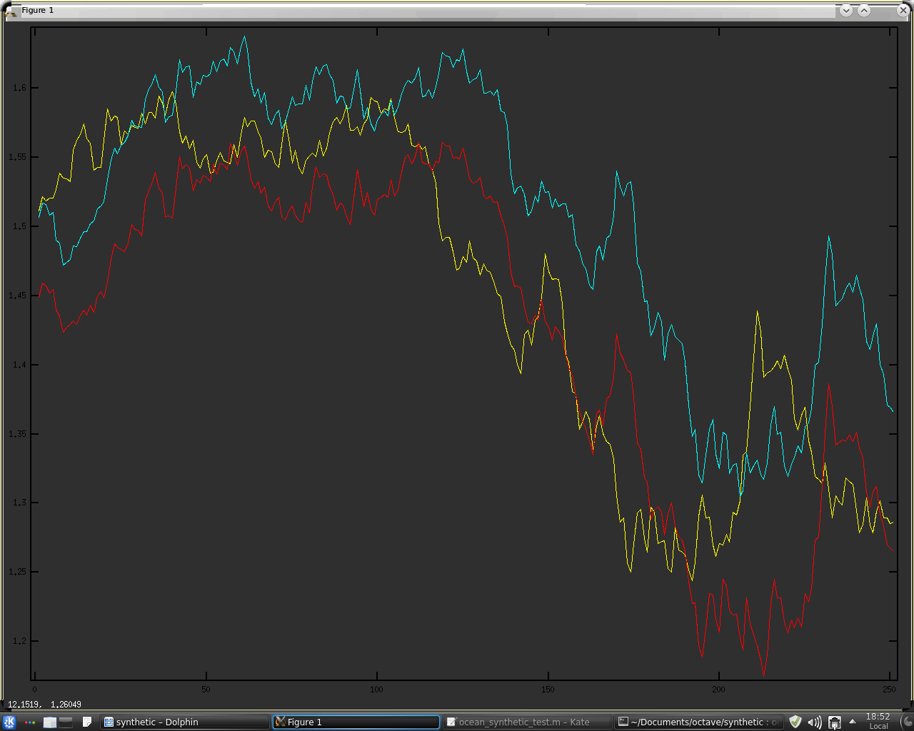
The basic premise, taken from Brownian motion, is that the natural log of price changes, on average, at a rate proportional to the square root of time. Take, for example, a period of 5 leading up to the "current bar." If we take a 5 period simple moving average of the absolute differences of the log of prices over this period, we get a value for the average 1 bar price movement over this period. This value is then multiplied by the square root of 5 and added to and subtracted from the price 5 days ago to get an upper and lower bound for the current bar. If the current bar lies between the bounds, we say that price movement over the last 5 periods is consistent with Brownian motion and declare an absence of trend, i.e. a sideways market. If the current bar lies outside the bounds, we declare that price movement over the last 5 bars is not consistent with Brownian motion and that a trend is in force, either up or down depending on which bound the current bar is beyond. The following 3 charts show this concept in action, for consecutive periods of 5, 13 and 21, taken from the Fibonacci Sequence:

where yellow is the closing price, blue is the upper bound and red the lower bound. It is easy to imagine many uses for this in terms of indicator creation, but I intend to use the bounds to assign a score of price randomness/trendiness over various combined periods to assign price movement to bins for subsequent Monte Carlo creation of synthetic price series. Interested readers are invited to read the above linked Creation of Synthetic Data post for a review of this methodology.

The rough working Octave code that produced the above charts is given below.

clear all

data = load("-ascii","eurusd") ;
% length = input( 'Enter length of look back for calculations: ' ) ;
% sq_rt = sqrt( length ) ;
close = data(:,7) ;
abslogdiff = abs( [ 0 ; diff( log(close) ) ] ) ;

lngth = 3 ;
sq_rt = sqrt( lngth ) ;
sma3 = sma(abslogdiff,lngth) ;
ub = exp(shift(log(close),lngth).+(sma3.*sq_rt)) ;
lb = exp(shift(log(close),lngth).-(sma3.*sq_rt)) ;

all_ub = ub ;
all_lb = lb ;

lngth = 5 ;
sq_rt = sqrt( lngth ) ;
sma5 = sma(abslogdiff,5) ;
ub = exp(shift(log(close),lngth).+(sma5.*sq_rt)) ;
lb = exp(shift(log(close),lngth).-(sma5.*sq_rt)) ;

all_ub = all_ub .+ ub ;
all_lb = all_lb .+ lb ;

lngth = 8 ;
sq_rt = sqrt( lngth ) ;
sma8 = sma(abslogdiff,lngth) ;
ub = exp(shift(log(close),lngth).+(sma8.*sq_rt)) ;
lb = exp(shift(log(close),lngth).-(sma8.*sq_rt)) ;

all_ub = all_ub .+ ub ;
all_lb = all_lb .+ lb ;

lngth = 13 ;
sq_rt = sqrt( lngth ) ;
sma13 = sma(abslogdiff,lngth) ;
ub = exp(shift(log(close),lngth).+(sma13.*sq_rt)) ;
lb = exp(shift(log(close),lngth).-(sma13.*sq_rt)) ;

all_ub = all_ub .+ ub ;
all_lb = all_lb .+ lb ;

lngth = 21 ;
sq_rt = sqrt( lngth ) ;
sma21 = sma(abslogdiff,lngth) ;
ub = exp(shift(log(close),lngth).+(sma21.*sq_rt)) ;
lb = exp(shift(log(close),lngth).-(sma21.*sq_rt)) ;

all_ub = ( all_ub .+ ub ) ./ 5 ;
all_lb = ( all_lb .+ lb ) ./ 5 ;

 plot(close(1850:2100,1),'y',ub(1850:2100,1),'c',lb(1850:2100,1),'r')
%plot(close,'y',ub,'c',lb,'r')

Change of Direction in Neural Net Training.

Up till now when training my neural net classifier I have been using what I call my "idealised" data, which is essentially a model for prices comprised of a sine wave along with a linear trend. In my recent work on Savitzky-Golay filters I wanted to increase the amount of available training data but have run into a problem - the size of my data files has become so large that I'm exhausting the memory available to me in my Octave software install. To overcome this problem I have decided to convert my NN training to an online regime rather than loading csv data files for mini-batch gradient descent training - in fact what I envisage doing would perhaps be best described as online mini-batch training.

To do this will require a fairly major rewrite of my data generation code and I think I will take the opportunity to make this data generation more realistic than the sine wave and trend model I am currently using. Apart from the above mentioned memory problem, this decision has been prompted by an e-mail exchange I have recently had with a reader of this blog and some online reading I have recently been doing, such as mixed regime simulation, training a simple neural network to recognise different regimes in financial time series, neural networks in trading, random subspace optimisation and profitable hidden and markovian coupling. At the moment it is my intention to revisit my earlier posts here and here and use/extend the ideas contained therein. This means that for the nearest future my work on Savitzky-Golay filters is temporarily halted.

Code refactoring didn't work.

In my previous post I said that I was going to refactor code to use my existing, trained classification neural net with Savitzky-Golay filter inputs in the hope that this might show some improvement. I have to report that this was an abysmal failure and I suppose it was a bit naive to have ever expected that it would work. It looks like I will have to explicitly train a new neural network to take advantage of Savitzky-Golay filter features.

Update on Savitzky-Golay Filters

For the past couple of weeks I have been playing around with Savitzky-Golay filters with a hope of creating a moving endpoint regression line as a form of zero lag smoothing, but unfortunately I have been unable to come up with anything that is remotely satisfying and I think I'm going to abandon this for now. My view at the moment is that SG filters' utility, for my purposes at least, is limited to feature extraction via the polynomial coefficients to get the 2nd, 3rd and 4th derivatives as inputs for my Neural net classifier.

To do this will require a time consuming retraining period, so before I embark on this I'm going to use what I think will be an immediately useful SG filter application. In a previous post readers can see three screenshots of moving windows of my idealised price series with SG filters overlaid. The SG filters follow these windowed "prices" so closely that I think SG filters more or less == windowed idealised prices and features derived there from. However, when it comes to applying my currently trained NN the features are derived from the noisy real prices seen in the video of the above linked post. What I intend to do wherever possible is to use a cubic SG filter applied to windowed prices and then derive input features from the SG filter values. Effectively what I will be doing is coercing real prices into smooth curves that far more closely resemble the idealised prices my NN was trained on. The advantage of this is that I will not have to retrain the NN, but only refactor my feature extraction code for use on real prices to this end. The hope is, of course, that this tweak will result in vastly improved performance to the extent that I will not need to consider future classifier NN retraining with polynomial derivatives and can proceed directly to training other NNs.

Finally, on a related note, I have recently been directed to this paper, which has some approaches to time series classification that I might incorporate in future NN training. Fig. 5 on page 9 shows six examples of time series classification categories. My idealised prices categories currently encompass what is described in the paper as "Cyclic," "Increasing Trend" and "Decreasing Trend." I shall have to consider whether it might be useful to extend my categories to include "Normal," "Upward Shift" and "Downward Shift." 

Review of Quantpedia.com

I was recently contacted and asked if I wouldn't mind writing a short review of the Quantpedia website in return for complimentary access to that site's premium section, and I am happy to do so. Readers can get a flavour of the website by perusing the free content that is available in the Screener tab and reading the Home, About and How We Do It tabs. Since these are readily accessible by any visitor to the site, this review will concentrate purely on the content available in the premium section.

The thing that strikes me is the wide and eclectic range of studies available, which can be easily seen by clicking on the keywords dropdown box on the screener tab. There is something for almost all trading styles and I would be surprised if a visitor to the premium section found nothing of value. As always the devil is in the details, and of course I haven't read anywhere near all the information that is available in the various studies, but a brief visual overview of the various studies' performance taken from Quantpedia's screener page is provided in the scatterchart below:

(n.b. Those studies that lie exactly on the y-axis (volatility = 0%) do not have no volatility, but no % figure for volatility was given in the screener.)

As can be seen there are some impressive performers, which are fully disclosed in the premium section. A few studies, irrespective of performance, did catch my immediate attention. Firstly, there are a couple of studies that look at lunar effects in stock markets and precious metals. Long time readers of this blog will know that some time back I did a series of tests on the Delta Phenomenon, which is basically a lunar effect model of price turning points. The conclusion of the tests I conducted was that the Delta Phenomenon did have statistically significant predictive ability. The above mentioned studies come to the same conclusion with regard to lunar effects, although via a different testing methodology. It is comforting to have one's own research conclusions confirmed by independent researchers, and it's a valuable resource to be able to see how other researchers approach the testing of similar market hypotheses.

Secondly, there is a study on using Principal Components Analysis to characterise the current state of the market. This is very much in tune with what I'm working on at the moment with my neural net market classifier, and the idea of using PCA as an input is a new one to me and one that I shall almost certainly look into in more detail.

This second point I think neatly sums up the main value of the studies on the Quantpedia site - they can give you new insights as to how one might develop one's own trading system(s), with the added benefit that the idea is not a dead end because it has already been tested by the original paper's authors and the Quantpedia site people. You could also theoretically just take one of the studies as a stand alone system and tweak it to suit your own needs, or add it as a form of diversification to an existing set of trading systems. Given the wide range of studies available, this would be a much more robust form of diversification than merely adjusting a look back length, parameter value or some other such cosmetic adjustment.

In conclusion, since I can appreciate the value in the Quantpedia site, I would like to thank Martin Nizny of Quantpedia for extending me the opportunity to review the premium section of the site.

Savitzky-Golay Filters in Action

As a first step in investigating SG filters I have simply plotted them on samples of my idealised time series data, three samples shown below:

where the underlying "price" is cyan, and the 3rd, 4th, 5th, 6th and 7th order SG fits are blue, red, magenta, green and yellow respectively. As can be seen, 5th order and above perfectly match the underlying price to the extent that the cyan line is completely obscured.

Repeating the above on real prices (ES-mini close) is shown in the video below:

Firstly, the thing that is immediately apparent is that real prices are more volatile than my idealised price series, a statement of the obvious perhaps, but it has led me to reconsider how I model my idealised price series. However, there are times when the patterns of the SG filters on real prices converge to almost identically resemble the patterns of SG filters on my idealised prices. This observation encourages me to continue to look at applying SG filters for my purposes. How I plan to use SG filters and modify my idealised price series will be the subject of my next post.

Savitzky-Golay Filter Convolution Coefficients

My investigation so far has had me reading General Least Squares Smoothing And Differentiation By The Convolution Method, a paper in the reference section of the Wikipedia page on Savitzky-Golay filters. In this paper there is Pascal code for calculating the convolution coefficients for a Savitzky-Golay filter, and in the code box below is my C++ translation of this Pascal code. Nb, due to formatting issues the symbol "<" appears as ampersand lt semi-colon in this code.

// Calculate Savitzky-Golay Convolution Coefficients
#include 
using namespace std;

double GenFact (int a, int b)
{ // calculates the generalised factorial (a)(a-1)...(a-b+1)

  double gf = 1.0 ;
  
  for ( int jj = (a-b+1) ; jj < a+1 ; jj ++ ) 
  {
    gf = gf * jj ; 
  }  
    return (gf) ;
    
} // end of GenFact function

double GramPoly( int i , int m , int k , int s )
{ // Calculates the Gram Polynomial ( s = 0 ), or its s'th
  // derivative evaluated at i, order k, over 2m + 1 points
  
double gp_val ;  

if ( k > 0 )
{   
gp_val = (4.0*k-2.0)/(k*(2.0*m-k+1.0))*(i*GramPoly(i,m,k-1,s) + s*GramPoly(i,m,k-1.0,s-1.0)) - ((k-1.0)*(2.0*m+k))/(k*(2.0*m-k+1.0))*GramPoly(i,m,k-2.0,s) ;
}
else
{  
  if ( ( k == 0 ) && ( s == 0 ) )
  {
     gp_val = 1.0 ;
  }     
  else
  {
     gp_val = 0.0 ;
  } // end of if k = 0 & s = 0  
} // end of if k > 0

return ( gp_val ) ;

} // end of GramPoly function

double Weight( int i , int t , int m , int n , int s )
{ // calculates the weight of the i'th data point for the t'th Least-square
  // point of the s'th derivative, over 2m + 1 points, order n

double sum = 0.0 ;

for ( int k = 0 ; k < n + 1 ; k++ )
{
sum += (2.0*k+1.0) * ( GenFact(2.0*m,k) / GenFact(2.0*m+k+1.0,k+1.0) ) * GramPoly(i,m,k,0) * GramPoly(t,m,k,s) ;    
} // end of for loop

return ( sum ) ;
                                               
} // end of Weight function

int main ()
{ // calculates the weight of the i'th data point (1st variable) for the t'th   Least-square point (2nd variable) of the s'th derivative (5th variable), over 2m + 1 points (3rd variable), order n (4th variable)
  
  double z ;
  
  z = Weight (4,4,4,2,0) ; // adjust input variables for required output
  
  cout << "The result is " << z ;
  
  return 0 ;
}

Whilst I don't claim to understand all the mathematics behind this, the use of the output of this code is conceptually not that much more difficult than a FIR filter, i.e. multiply each value in a look back window by some coefficient, except that a polynomial of a given order is being least squares fit to all points in the window rather than, for example, an average of all the points being calculated. The code gives the user the ability to calculate the value of the polynomial at each point in the window, or its derivative(s) at that point.

I would particularly draw readers' attention to the derivative(s) link above. On this page there is an animation of the slope (1st derivative) of a waveform. If this were to be applied to a price time series the possible applications become apparent: a slope of zero will pick out local highs and lows to identify local support and resistance levels; an oscillator zero crossing will give signals to go long or short; oscillator peaks will give signals to tighten stops or place profit taking orders. And why stop there? Why not use the second derivative as a measure of the acceleration of a price move? And how about the jerk and the jounce of a price series? I don't know about readers, but I have never seen a trading article, forum post or blog talk about the jerk and jounce of price series. Of course, if one were to plot all these as indicators I'm sure it would just be confusing and nigh impossible to come up with a cogent rule set to trade with. However, one doesn't have to do this oneself, and this is what I was alluding to in my earlier post when I said that the Savitzky-Golay framework might provide unique and informative inputs to my neural net trading system. Providing enough informative data is available for training, the rule set will be encapsulated within the weights of any trained neural net.