Thursday, 18 June 2020

More Work on RVFL Networks

Back in November last year I posted about Random Vector Functional Link (RVFL) networks here and here. Since then, along with my recent work on Oanda's API Octave functions and Market/Volume Profile visualisation, I have continued looking at RVFL networks and this post is an update on this work.

The "random" in RVFL means random initialisation of weights that are then fixed. It seems to me that it might be possible to do better than random by having some principled way of weight initialisation. To this end I have used the Penalised MATLAB Toolbox on features derived from my ideal cyclic tau embedding function to at first train a Generalized Linear Model with the Lasso penalty and then the Ridge penalty over thousands of sets of Monte Carlo generated, ideal cyclic prices and such prices with trends. The best weights for each set of prices were recorded in an array and then the mean weight (and standard deviation) taken. This set of mean weights is intended to replace the random weights in a RVFL network designed to predict the probability of "price" being at a cyclic turning point using the above cyclic tau embedding features.

Of course these weights could be considered a trained model in and of themselves, and the following screenshots show "out of sample" performance on Monte Carlo generated ideal prices that were not used in the training of the mean weights.
The black line is the underlying cyclic price and the red, blue and green lines are the mean weight model probabilities for cyclic peaks, troughs or neither respectively. Points where the peak/trough probabilities exceed the neither probabilities are marked by the red and blue vertical lines. Similarly, we have prices trending up in a cyclic fashion
and also trending down
In the cases of the last two trending markets only the swing highs and lows are indicated. The reason for this is that during training, based on my "expert knowledge" of the cyclic tau features used, it is unreasonable to expect these features to accurately capture the end of an up leg in a bull trend or the end of a down leg in a bear trend - hence these were not presented as a positive class during training.

As I said above the motivation for this is to get a more meaningful hidden layer in a RVFL network. This hidden layer will consist of seven Sigmoid functions which each give a probability of price being at or not being at a cyclic turn, conditional upon the type of market the input weights were trained on.

More in due course.

Saturday, 6 June 2020

Downloading FX Pairs via Oanda API to Calculate Currency Strength Indicator

In the past I have posted a series of blog posts about a Currency Strength Indicator (here, here, here and here). This blog post gives an Octave function to use Oanda's API to download all the 10 minute OHLC data required to calculate the above strength indicators on the 10 minute time frame.
## Copyright (C) 2020 dekalog
## 
## This program is free software: you can redistribute it and/or modify it
## under the terms of the GNU General Public License as published by
## the Free Software Foundation, either version 3 of the License, or
## (at your option) any later version.
## 
## This program is distributed in the hope that it will be useful, but
## WITHOUT ANY WARRANTY; without even the implied warranty of
## MERCHANTABILITY or FITNESS FOR A PARTICULAR PURPOSE.  See the
## GNU General Public License for more details.
## 
## You should have received a copy of the GNU General Public License
## along with this program.  If not, see
## .

## -*- texinfo -*- 
## @deftypefn {} {@var{retval} =} get_currency_index_10m_pairs()
##
## This function gets the date and time value of the last currency index update for
## 10 minute bars by reading the last line of the file at:
##
## "/home/path/to/file"
##
## and then downloads all the currencies required to calculate new values for
## new currency index calculations, via looped Oanda API calls. 
## 
##The RETVAL is a matrix of GMT dates in the form
## YYYY:MM:DD:HH:MM in the first 5 columns, followed by the 45 required
## currency candlestick close values.
##
## @seealso{}
## @end deftypefn

## Author: dekalog 
## Created: 2020-06-01

function retval = get_currency_index_10m_pairs()
 
## cell array of currency crosses to iterrate over to get the complete set 
## of currency crosses to create a currency index
iter_vec = {'AUD_CAD','AUD_CHF','AUD_HKD','AUD_JPY','AUD_NZD','AUD_SGD',...
'AUD_USD','CAD_CHF','CAD_HKD','CAD_JPY','CAD_SGD','CHF_HKD','CHF_JPY',...
'EUR_AUD','EUR_CAD','EUR_CHF','EUR_GBP','EUR_HKD','EUR_JPY','EUR_NZD',...
'EUR_SGD','EUR_USD','GBP_AUD','GBP_CAD','GBP_CHF','GBP_HKD','GBP_JPY',...
'GBP_NZD','GBP_SGD','GBP_USD','HKD_JPY','NZD_CAD','NZD_CHF','NZD_HKD',...
'NZD_JPY','NZD_SGD','NZD_USD','SGD_CHF','SGD_HKD','SGD_JPY','USD_CAD',...
'USD_CHF','USD_HKD','USD_JPY','USD_SGD'} ;

## read last line of current 10min_currency_indices
unix_command = [ "tail -1" , " " , "/home/path/to/file" ] ;
[ ~ , data ] = system( unix_command ) ;
data = strsplit( data , ',' ) ; ## gives a cell arrayfun of characters
## zero pad singular month representations, i.e. 1 to 01
if ( numel( data{ 2 } == 1 ) )
data{ 2 } = [ '0' , data{ 2 } ] ;
endif
## and also zero pad singular dates
if ( numel( data{ 3 } == 1 ) )
data{ 3 } = [ '0' , data{ 3 } ] ;
endif
## and also zero pad singular hours
if ( numel( data{ 4 } == 1 ) )
data{ 4 } = [ '0' , data{ 4 } ] ;
endif
## and also zero pad singular minutes
if ( numel( data{ 5 } == 1 ) )
data{ 5 } = [ '0' , data{ 5 } ] ;
endif
 
## set up the headers
Hquery = [ 'curl -s -H "Content-Type: application/json"' ] ; ## -s is silent mode for Curl for no paging to terminal
Hquery = [ Hquery , ' -H "Authorization: Bearer XXXXXXXXXXXXXXXXXXXXXXXXXXXXXXXXXXXXXXXXXXXXXXXXXXXXXXXXXXXXX"' ] ;
query_begin = [ Hquery , ' "https://api-fxtrade.oanda.com/v3/instruments/' ] ;

## get time from last line of data
query_time = [ data{1} , '-' , data{2} , '-' , data{3} , 'T' , data{4} , '%3A' , data{5} , '%3A00.000000000Z&granularity=M10"' ] ;

## initialise with AUD_CAD
## construct the API call for particular cross
query = [ query_begin , iter_vec{ 1 } , '/candles?includeFirst=true&price=M&from=' , query_time ] ;
## call to use external Unix systems/Curl and return result
[ ~ , ret_JSON ] = system( query , RETURN_OUTPUT = 'TRUE' ) ;
## convert the returned JSON object to Octave structure
S = load_json( ret_JSON ) ;
## parse the returned structure S
if ( strcmp( fieldnames( S( 1 ) ) , 'errorMessage' ) == 0 ) ## no errorMessage in S
end_ix = numel( S.candles ) ; ## how many candles?
if ( S.candles{ end }.complete == 0 ) end_ix = end_ix - 1 ; endif ## account for incomplete candles
## create retval
retval = zeros( end_ix , 50 ) ; ## 45 currencies plus YYYY:MM:DD:HH:MM columns
for ii = 1 : end_ix
 date_time = strsplit( S.candles{ ii }.time , { '-' , 'T' , ':' } ) ;
 retval( ii , 1 ) = str2double( date_time( 1 , 1 ) ) ; ## year
 retval( ii , 2 ) = str2double( date_time( 1 , 2 ) ) ; ## month
 retval( ii , 3 ) = str2double( date_time( 1 , 3 ) ) ; ## day
 retval( ii , 4 ) = str2double( date_time( 1 , 4 ) ) ; ## hour
 retval( ii , 5 ) = str2double( date_time( 1 , 5 ) ) ; ## min
 retval( ii , 6 ) = str2double( S.candles{ ii }.mid.c ) ; ## candle close price 
endfor ## end of ii loop
else
error( 'Initialisation with AUD_CAD has failed.' ) ; 
endif ## end of strcmp if

for ii = 2 : numel( iter_vec )
## construct the API call for particular cross
query = [ query_begin , iter_vec{ ii } , '/candles?includeFirst=true&price=M&from=' , query_time ] ;
## call to use external Unix systems/Curl and return result
[ ~ , ret_JSON ] = system( query , RETURN_OUTPUT = 'TRUE' ) ;
## convert the returned JSON object to Octave structure
S = load_json( ret_JSON ) ;
## parse the returned structure S
if ( strcmp( fieldnames( S( 1 ) ) , 'errorMessage' ) == 0 ) ## no errorMessage in S
end_ix = numel( S.candles ) ; ## how many candles?
if ( S.candles{ end }.complete == 0 ) end_ix = end_ix - 1 ; endif ## account for incomplete candles
temp_retval = zeros( end_ix , 6 ) ;
for jj = 1 : end_ix
 date_time = strsplit( S.candles{ jj }.time , { '-' , 'T' , ':' } ) ;
 temp_retval( jj , 1 ) = str2double( date_time( 1 , 1 ) ) ; ## year
 temp_retval( jj , 2 ) = str2double( date_time( 1 , 2 ) ) ; ## month
 temp_retval( jj , 3 ) = str2double( date_time( 1 , 3 ) ) ; ## day
 temp_retval( jj , 4 ) = str2double( date_time( 1 , 4 ) ) ; ## hour
 temp_retval( jj , 5 ) = str2double( date_time( 1 , 5 ) ) ; ## min
 temp_retval( jj , 6 ) = str2double( S.candles{ jj }.mid.c ) ; ## candle close price  
endfor ## end of jj loop

## checks dates and times allignment before writing to retval
date_time_diffs_1 = setdiff( retval( : , 1 : 5 ) , temp_retval( : , 1 : 5 ) , 'rows' ) ; 
date_time_diffs_2 = setdiff( temp_retval( : , 1 : 5 ) , retval( : , 1 : 5 ) , 'rows' ) ;

 if ( isempty( date_time_diffs_1 ) && isempty( date_time_diffs_2 ) ) 
 ## there are no differences between retval dates and temp_retval dates 
 retval( : , ii + 5 ) = temp_retval( : , 6 ) ;
 
 elseif ( ~isempty( date_time_diffs_1 ) || ~isempty( date_time_diffs_2 ) )
 ## implies a difference between the date_times of retval and temp_retval, so merge them
 
 dn_retval = datenum( [ retval(:,1) , retval(:,2) , retval(:,3) , retval(:,4) , retval(:,5) ] ) ;
 dn_temp_retval = datenum( [ temp_retval(:,1) , temp_retval(:,2) , temp_retval(:,3) , temp_retval(:,4) , temp_retval(:,5) ] ) ;
 new_dn = unique( [ dn_retval ; dn_temp_retval ] ) ; new_date_vec = datevec( new_dn ) ; new_date_vec( : , 6 ) = [] ; 
 new_retval = [ new_date_vec , zeros( size( new_date_vec , 1 ) , 45 ) ] ;
 [ TF , S_IDX ] = ismember( new_retval( : , 1 : 5 ) , retval( : , 1 : 5 ) , 'rows' ) ;
 TF_ix = find( TF ) ; new_retval( TF_ix , 6 : end ) = retval( : , 6 : end ) ;
 [ TF , S_IDX ] = ismember( new_retval( : , 1 : 5 ) , temp_retval( : , 1 : 5 ) , 'rows' ) ;
 TF_ix = find( TF ) ; new_retval( TF_ix , ii + 5 ) = temp_retval( : , 6 ) ; 
 retval = new_retval ; 
 clear new_retval new_dn dn_temp_retval dn_retval date_time_diffs_1 date_time_diffs_2 ;
 
 else 
 error( 'Mismatch between dates and times for writing to retval.' ) ; 
 endif ## TF == S_IDX check

endif ## end of strcmp if

endfor ## ii loop

endfunction
At the moment there are almost 50 separate API calls nested within a loop, which of course is non-vectorised and inefficient, and if I find out how to make a batch API call to do this I shall rewrite the function.

This function is called in a script which uses the output matrix "retval" to then calculate the various currency strengths as outlined in the above linked posts. The total running time for this script is approximately 40 seconds from first call to appending to the index file on disk. I wrote this function to leverage my new found Oanda API knowledge to avoid having to accumulate an ever growing set of files on disk containing the raw 10 minute data.

I hope readers find this useful.

Wednesday, 20 May 2020

An Improved Volume Profile Chart with Levels

Without much ado, here is the code
## Copyright (C) 2020 dekalog
## 
## This program is free software: you can redistribute it and/or modify it
## under the terms of the GNU General Public License as published by
## the Free Software Foundation, either version 3 of the License, or
## (at your option) any later version.
## 
## This program is distributed in the hope that it will be useful, but
## WITHOUT ANY WARRANTY; without even the implied warranty of
## MERCHANTABILITY or FITNESS FOR A PARTICULAR PURPOSE.  See the
## GNU General Public License for more details.
## 
## You should have received a copy of the GNU General Public License
## along with this program.  If not, see
## .

## -*- texinfo -*- 
## @deftypefn {} {@var{retval} =} market_profile_plot (@var{cross}, @var{n_bars})
##
## Plot a Market Profile Chart of CROSS of the last N_BARS.
##
## @seealso{}
## @end deftypefn

## Author: dekalog 
## Created: 2020-05-11

function market_profile_plot( curr_cross , n_days )

pkg load statistics ; 
cd /path/to/data/folder ;
price_name = tolower( curr_cross ) ;

if ( strcmp( price_name , 'aud_jpy' ) || strcmp( price_name , 'eur_jpy' ) || strcmp( price_name , 'gbp_jpy' ) || ...
     strcmp( price_name , 'usd_jpy' ) )
 tick_size = 0.001 ;
 round_digit = 3 ;
elseif ( strcmp( price_name , 'xau_usd' ) )
 tick_size = 0.1 ;
 round_digit = 1 ;
elseif ( strcmp( price_name , 'xag_usd' ) )
 tick_size = 0.01 ;
 round_digit = 2 ; 
else
 tick_size = 0.0001 ;
 round_digit = 4 ;
endif

## get price data of *_ohlc_10m
unix_command = [ "wc" , " " , "-l" , " " , [ price_name , '_ohlc_10m' ] ] ;
## the 'wc' with '-l' flag command counts the number of lines in [ price_name , '_ohlc_20m' ] } 
[ ~ , system_out ] = system( unix_command ) ;
cstr = strsplit( system_out , " " ) ; 
lines_in_file = str2double( cstr( 1 , 1 ) ) ;

## read *_ohlc_10m file
price_data = dlmread( [ price_name , '_ohlc_10m' ] , ',' , [ lines_in_file - ( n_days * 144 + 18 ) , 0 , lines_in_file , 21 ] ) ;
## get the earliest London open on a Sunday, if any
sun_open_ix = find( ( price_data( : , 11 ) == 1 ) .* ( price_data( : , 9 ) == 22 ) .* ( price_data( : , 10 ) == 0 ) ) ;
## get weekday closes
end_ix = find( ( price_data( : , 15 ) == 16 ) .* ( price_data( : , 16 ) == 50  ) ) ;
delete_ix = unique( [ sun_open_ix ; end_ix ] ) ;
## delete uuwanted data
price_data( 1 : delete_ix( 1 ) , : ) = [] ; end_ix = end_ix .- delete_ix( 1 ) ; open_ix = end_ix .+ 1 ; 
end_ix( end_ix == 0 ) = [] ; end_ix( end_ix > size( price_data , 1 ) ) = [] ;
open_ix( open_ix == 0 ) = [] ; open_ix( open_ix > size( price_data , 1 ) ) = [] ;

## give names to data
open = price_data(:,18) ; high = price_data(:,19) ; low = price_data(:,20) ; close = price_data(:,21) ; vol = price_data(:,22) ;
high_round = floor( high ./ tick_size .+ 0.5 ) .* tick_size ;
low_round = floor( low ./ tick_size .+ 0.5 ) .* tick_size ;
max_tick_range = max( high_round .- low_round ) / tick_size ;
upper_val = high ; lower_val = low ;

## create y and x axes for chart
y_max = max( high_round ) + max_tick_range * tick_size ;
y_min = min( low_round ) - max_tick_range * tick_size ;
y_ax = ( y_min : tick_size : y_max )' ;
end_x_ax_freespace = 5 ;

## create container
all_vp = zeros( n_days , numel( y_ax ) ) ; all_mp = all_vp ;

if ( n_days == 1 )

[ all_vp(1,:) , vp_val ] = pcolor_background( y_ax , high , low , vol , tick_size ) ;
vp_z = repmat( all_vp( 1 , : ) , numel( high ) + end_x_ax_freespace , 1 ) ;
lower_val( : ) = vp_val( 1 ) ; upper_val( : ) = vp_val( 2 ) ; 

elseif ( n_days >= 2 )

vp_z = zeros( numel( high ) + end_x_ax_freespace , size( all_vp , 2 ) ) ;

 for ii = 1 : numel( end_ix ) 
 [ all_vp(ii,:) , vp_val ] = pcolor_background( y_ax , high(open_ix(ii):end_ix(ii)) , low(open_ix(ii):end_ix(ii)) , ...
                                                        vol(open_ix(ii):end_ix(ii)) , tick_size ) ;
 vp_z(open_ix(ii):end_ix(ii),:) = repmat( all_vp(ii,:)./max(all_vp(ii,:)) , numel( high(open_ix(ii):end_ix(ii)) ) , 1 ) ;
 lower_val( open_ix(ii) : end_ix(ii) ) = vp_val( 1 ) ; upper_val( open_ix(ii) : end_ix(ii) ) = vp_val( 2 ) ;
 endfor

[ all_vp(end,:) , vp_val ] = pcolor_background( y_ax , high(open_ix(end):end) , low(open_ix(end):end) , ...
                                                         vol(open_ix(end):end) , tick_size ) ;
vp_z( open_ix( end ) : end , : ) = repmat( all_vp( end , : ) ./ max( all_vp( end , : ) ) , ...
                                            numel( high( open_ix( end ) : end ) ) + end_x_ax_freespace , 1 ) ;
lower_val( open_ix( end ) : end ) = vp_val( 1 ) ; upper_val( open_ix( end ) : end ) = vp_val( 2 ) ;
endif

## create the background ( best choices - viridis and ocean? )
x_ax = ( 1 : 1 : numel( open ) + end_x_ax_freespace )' ;
colormap( 'viridis' ) ; figure( 10 ) ; pcolor( x_ax , y_ax , vp_z' ) ; shading interp ; axis tight ;

## plot the individual volume profiles
hold on ;

scale_factor = ( 1 / max(max(all_vp) ) ) * 72 ;
for ii = 1 : numel( open_ix )
figure( 10 ) ; fill( all_vp( ii , : ) .* scale_factor .+ open_ix( ii ) , y_ax' , [99;99;99]./255 ) ;
endfor

## plot candlesticks
figure( 10 ) ; candle_mp( high , low , close , open ) ;

## plot upper and lower boundaries of value area
hold on ; figure( 10 ) ; plot( lower_val , 'b' , 'linewidth' , 2 , upper_val , 'r' , 'linewidth' , 2 ) ; hold off ;

## Plot vertical lines for London open at 7am
london_ix = find( ( price_data( : , 9 ) == 7 ) .* ( price_data( : , 10 ) == 0 ) ) ;
if ( ~isempty( london_ix ) )
 for ii = 1 : numel( london_ix )
  figure( 10 ) ; vline( london_ix( ii ) , 'g' ) ;
 endfor
endif

endfunction
which calls this
## Copyright (C) 2020 dekalog
## 
## This program is free software: you can redistribute it and/or modify it
## under the terms of the GNU General Public License as published by
## the Free Software Foundation, either version 3 of the License, or
## (at your option) any later version.
## 
## This program is distributed in the hope that it will be useful, but
## WITHOUT ANY WARRANTY; without even the implied warranty of
## MERCHANTABILITY or FITNESS FOR A PARTICULAR PURPOSE.  See the
## GNU General Public License for more details.
## 
## You should have received a copy of the GNU General Public License
## along with this program.  If not, see
## .

## -*- texinfo -*- 
## @deftypefn {} {@var{vp_z}, @var{vp_val} =} pcolor_background (@var{y_ax}, @var{high}, @var{low}, @var{vol}, @var{tick_size})
##
## @seealso{}
## @end deftypefn

## Author: dekalog 
## Created: 2020-05-13

function [ vp_z , vp_val ] = pcolor_background ( y_ax , high , low , vol , tick_size )

vp_z = zeros( 1 , numel( y_ax ) ) ; ##tpo_z = vp_z ;
vol( vol <= 1 ) = 2 ; ## no single point vol distributions
vp_val = zeros( 2 , 1 ) ;

 for ii = 1 : numel( high )

 ## the volume profile, vp_z
 ticks = norminv( linspace(0,1,vol(ii)+2) , (high(ii) + low(ii))/2 , (high(ii) - low(ii))*0.25 ) ;
 ticks = floor( ticks( 2 : end - 1 ) ./ tick_size .+ 0.5 ) .* tick_size ;
 unique_ticks = unique( ticks ) ;

  if ( numel( unique_ticks ) > 1 )
  [ N , X ] = hist( ticks , unique( ticks ) ) ;
  [ ~ , N_ix ] = max( N ) ; tick_ix = X( N_ix ) ;
  [ ~ , centre_tick ] = min( abs( y_ax .- tick_ix ) ) ;
  vp_z(1,centre_tick-N_ix+1:centre_tick+(numel(N)-N_ix)) = vp_z(1,centre_tick-N_ix+1:centre_tick+(numel(N)-N_ix)).+ N ;
  elseif ( numel( unique_ticks ) == 1 )
  [ ~ , centre_tick ] = min( abs( y_ax .- unique_ticks ) ) ;
  vp_z( 1 , centre_tick ) = vp_z( 1 , centre_tick ) + vol( ii ) ;
  endif

 endfor

[ ~ , vp_val_centre_ix ] = max( vp_z ) ;
sum_vp_cutoff = 0.7 * sum( vp_z ) ;
count = 1 ;

while ( count ~= 0 )
 
 sum_vp_z = sum( vp_z( max( vp_val_centre_ix - count , 1 ) : min( vp_val_centre_ix + count , numel( vp_z ) ) ) ) ;
 if ( sum_vp_z >= sum_vp_cutoff )
  vp_val( 1 , 1 ) = y_ax( max( vp_val_centre_ix - count , 1 ) ) ;             ## lower
  vp_val( 2 , 1 ) = y_ax( min( vp_val_centre_ix + count , numel( vp_z ) ) ) ; ## upper
  count = 0 ;
 else
  count = count + 1 ;
 endif

 endwhile

endfunction
and this
function hhh=vline(x,in1,in2)
% function h=vline(x, linetype, label)
% 
% Draws a vertical line on the current axes at the location specified by 'x'.  Optional arguments are
% 'linetype' (default is 'r:') and 'label', which applies a text label to the graph near the line.  The
% label appears in the same color as the line.
%
% The line is held on the current axes, and after plotting the line, the function returns the axes to
% its prior hold state.
%
% The HandleVisibility property of the line object is set to "off", so not only does it not appear on
% legends, but it is not findable by using findobj.  Specifying an output argument causes the function to
% return a handle to the line, so it can be manipulated or deleted.  Also, the HandleVisibility can be 
% overridden by setting the root's ShowHiddenHandles property to on.
%
% h = vline(42,'g','The Answer')
%
% returns a handle to a green vertical line on the current axes at x=42, and creates a text object on
% the current axes, close to the line, which reads "The Answer".
%
% vline also supports vector inputs to draw multiple lines at once.  For example,
%
% vline([4 8 12],{'g','r','b'},{'l1','lab2','LABELC'})
%
% draws three lines with the appropriate labels and colors.
% 
% By Brandon Kuczenski for Kensington Labs.
% brandon_kuczenski@kensingtonlabs.com
% 8 November 2001
if length(x)>1  % vector input
    for I=1:length(x)
        switch nargin
        case 1
            linetype='r:';
            label='';
        case 2
            if ~iscell(in1)
                in1={in1};
            end
            if I>length(in1)
                linetype=in1{end};
            else
                linetype=in1{I};
            end
            label='';
        case 3
            if ~iscell(in1)
                in1={in1};
            end
            if ~iscell(in2)
                in2={in2};
            end
            if I>length(in1)
                linetype=in1{end};
            else
                linetype=in1{I};
            end
            if I>length(in2)
                label=in2{end};
            else
                label=in2{I};
            end
        end
        h(I)=vline(x(I),linetype,label);
    end
else
    switch nargin
    case 1
        linetype='r:';
        label='';
    case 2
        linetype=in1;
        label='';
    case 3
        linetype=in1;
        label=in2;
    end


    g=ishold(gca);
    hold on
    y=get(gca,'ylim');
    h=plot([x x],y,linetype);
    if length(label)
        xx=get(gca,'xlim');
        xrange=xx(2)-xx(1);
        xunit=(x-xx(1))/xrange;
        if xunit<0 .8="" code="" color="" else="" end="" g="=0" get="" h="" handlevisibility="" hhh="h;" hold="" if="" label="" nargout="" off="" set="" tag="" text="" vline="" x-.05="" x="" xrange="" y="">
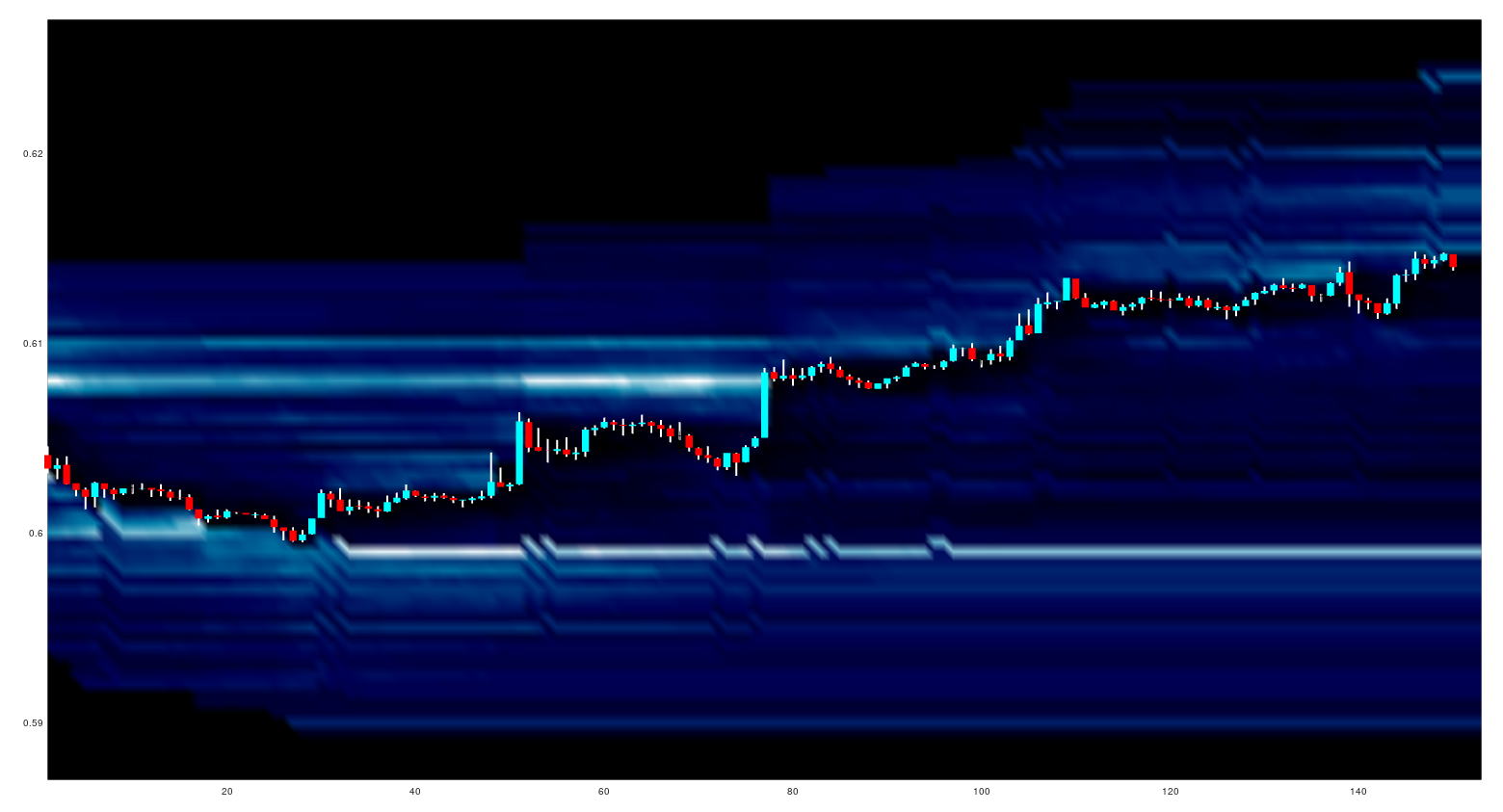
and produces charts such as this,
which is a 10 minute ohlc chart of the last 3 days, including "today's" ongoing price action. The number of days is a function input, and the horizontal blue and red lines indicate the upper and lower extremes of the value area. The vertical green lines indicate the London opening bar (7am BST) and each set of levels ends at the New York closing bar (5pm EST).

Further examples are last 10 days
and last month
Enjoy!


Monday, 18 May 2020

A Volume Profile With Levels Chart

Just a quick post to illustrate the latest of my ongoing chart iterations which combines a levels chart, as I have recently been posting about, but with the addition of a refined methodology of creating the horizontal histograms to more clearly represent the volumes over distinct periods.
The main change is to replace the use of the Octave barh function with the fill function. A minimal working example of this plotting is given in the code box below.
## get price data of *_ohlc_10m
unix_command = [ "wc" , " " , "-l" , " " , [ price_name , '_ohlc_10m' ] ] ;
## the 'wc' with '-l' flag command counts the number of lines in [ price_name , '_ohlc_20m' ] } 
[ ~ , system_out ] = system( unix_command ) ;
cstr = strsplit( system_out , " " ) ; 
lines_in_file = str2double( cstr( 1 , 1 ) ) ;

## read *_ohlc_10m file
price_data = dlmread( [ price_name , '_ohlc_10m' ] , ',' , [ lines_in_file - n_bars , 0 , lines_in_file , 21 ] ) ;
open = price_data(:,18) ; high = price_data(:,19) ; low = price_data(:,20) ; close = price_data(:,21) ; vol = price_data(:,22) ;
high_round = floor( high ./ tick_size .+ 0.5 ) .* tick_size ;
low_round = floor( low ./ tick_size .+ 0.5 ) .* tick_size ;
max_tick_range = max( high_round .- low_round ) / tick_size ;

## create y and x axes for chart
y_max = max( high_round ) + max_tick_range * tick_size ;
y_min = min( low_round ) - max_tick_range * tick_size ;
y_ax = ( y_min : tick_size : y_max )' ;
end_x_ax_freespace = 5 ;

all_vp = zeros( 3 , numel( y_ax ) ) ;

all_vp( 1 , : ) = pcolor_background( y_ax , high(1:50) , low(1:50) , vol(1:50) , tick_size ) ;
all_vp( 2 , : ) = pcolor_background( y_ax , high(51:100) , low(51:100) , vol(51:100) , tick_size ) ;
all_vp( 3 , : ) = pcolor_background( y_ax , high(100:150) , low(100:150) , vol(100:150) , tick_size ) ;

vp_z = repmat( sum( all_vp , 1 ) , numel( high ) + end_x_ax_freespace , 1 ) ;

x_ax = ( 1 : 1 : numel( open ) + end_x_ax_freespace )' ;
colormap( 'viridis' ) ; figure( 20 ) ; pcolor( x_ax , y_ax , vp_z' ) ; shading interp ; axis tight ;

## plot the individual volume profiles
hold on ;
scale_factor = 0.18 ; 
fill( all_vp( 1 , : ) .* scale_factor , y_ax' , [99;99;99]./255 ) ; 
fill( all_vp( 2 , : ) .* scale_factor .+ 50 , y_ax' , [99;99;99]./255 ) ;
fill( all_vp( 3 , : ) .* scale_factor .+ 100 , y_ax' , [99;99;99]./255 ) ;

## plot candlesticks
candle_mp( high , low , close , open ) ;
hold off;
I hope readers find this new way of plotting profile charts useful - I certainly am pretty pleased with it.

Saturday, 16 May 2020

A Comparison of Charts

Earlier in May I posted about Market Profile with some charts and video. Further work on this has made me realise that my earlier post should more accurately be described as Volume Profile, so apologies to readers for that.

Another, similar type of chart I have seen described as a TPO chart (TPO stands for 'That Price Occurred' or ticked) and it is a simple matter to extend the code in the above linked post to create a TPO chart and below is the Octave function I have written to produce the backgrounds for both types of plot
## Copyright (C) 2020 dekalog
## 
## This program is free software: you can redistribute it and/or modify it
## under the terms of the GNU General Public License as published by
## the Free Software Foundation, either version 3 of the License, or
## (at your option) any later version.
## 
## This program is distributed in the hope that it will be useful, but
## WITHOUT ANY WARRANTY; without even the implied warranty of
## MERCHANTABILITY or FITNESS FOR A PARTICULAR PURPOSE.  See the
## GNU General Public License for more details.
## 
## You should have received a copy of the GNU General Public License
## along with this program.  If not, see
## .

## -*- texinfo -*- 
## @deftypefn {} {@var{background} =} pcolor_background (@var{y_ax}, @var{high}, @var{low}, @var{vol}, @var{tick_size})
##
## Creates a matrix, BACKGOUND, to be used by Market Profile plotting functions,
## which need a colour background matrix to be plotted by pcolor.
## 
## @seealso{}
## @end deftypefn

## Author: dekalog 
## Created: 2020-05-13

function [ vp_background , mp_background ] = pcolor_background ( y_ax , high , low , vol , tick_size )

vp_z = zeros( 1 , numel( y_ax ) ) ; mp_z = vp_z ;
vol( vol <= 1 ) = 2 ; ## no single point vol distributions

for ii = 1 : numel( high )

## the volume profile, vp_background
ticks = norminv( linspace(0,1,vol(ii)+2) , (high(ii) + low(ii))/2 , (high(ii) - low(ii))*0.25 ) ;
ticks = floor( ticks( 2 : end - 1 ) ./ tick_size .+ 0.5 ) .* tick_size ;
unique_ticks = unique( ticks ) ;

if ( numel( unique_ticks ) > 1 )
[ N , X ] = hist( ticks , unique( ticks ) ) ;
[ ~ , N_ix ] = max( N ) ; tick_ix = X( N_ix ) ;
[ ~ , centre_tick ] = min( abs( y_ax .- tick_ix ) ) ;
vp_z(1,centre_tick-N_ix+1:centre_tick+(numel(N)-N_ix)) = vp_z(1,centre_tick-N_ix+1:centre_tick+(numel(N)-N_ix)).+ N ;
elseif ( numel( unique_ticks ) == 1 )
[ ~ , centre_tick ] = min( abs( y_ax .- unique_ticks ) ) ;
vp_z( 1 , centre_tick ) = vp_z( 1 , centre_tick ) + vol( ii ) ;
endif

## the market profile, mp_background
[ ~ , ix_high ] = min( abs( y_ax .- high( ii ) ) ) ;
[ ~ , ix_low ] = min( abs( y_ax .- low( ii ) ) ) ;
mp_z( 1 , ix_low : ix_high ) = mp_z( 1 , ix_low : ix_high ) .+ 1 ;

endfor

vp_background = repmat( vp_z , numel( high ) , 1 ) ;
mp_background = repmat( mp_z , numel( high ) , 1 ) ;

endfunction
I have elected to still call the TPO plot a Market Profile plot as, from what I can make out, the tick count of the TPO is intended to be a surrogate for the original, cleared volume of Market Profile.

The above function is intended to provide a matrix input for the pcolor function, which internally scales the matrix to 0-1. Another idea I have had is to multiply the Volume Profile matrix and the Market Profile matrix together to get a normalised Combined Profile matrix. The animated GIF below shows all three.
It can be seen that there are subtle differences between them but that, on the whole, the results are similar.

More in due course.

Friday, 8 May 2020

A Second Orderbook Visualisation Chart

Below is code for a second way of charting ohlc price with Oanda's order book levels. First, the function loads the relevant data and plots the order book levels with Octave's pcolor function and then plots the price ohlc as candlesticks over the pcolor plot. The candlestick part of the function reuses some of the code I wrote for the financial package's candle plotting function.
## Copyright (C) 2020 dekalog
## 
## This program is free software: you can redistribute it and/or modify it
## under the terms of the GNU General Public License as published by
## the Free Software Foundation, either version 3 of the License, or
## (at your option) any later version.
## 
## This program is distributed in the hope that it will be useful, but
## WITHOUT ANY WARRANTY; without even the implied warranty of
## MERCHANTABILITY or FITNESS FOR A PARTICULAR PURPOSE.  See the
## GNU General Public License for more details.
## 
## You should have received a copy of the GNU General Public License
## along with this program.  If not, see
## .

## -*- texinfo -*- 
## @deftypefn {} candle_with_order_levels (@var{cross}, @var{n_bars})
##
## Plots a 20 minute candlestick chart of the most recent N_BARS of currency CROSS with
## the background highlighted with Oanda's historical orderbook levels for
## this CROSS.
##
## @seealso{candle,snake_and_canyon_plot}
## @end deftypefn

## Author: dekalog 
## Created: 2020-05-06

function candle_with_order_levels ( curr_cross , n_bars )

price_name = tolower( curr_cross ) ;

## get price data of *_ohlc_20m
unix_command = [ "wc" , " " , "-l" , " " , [ price_name , '_ohlc_20m' ] ] ;
## the 'wc' with '-l' flag command counts the number of lines in [ price_name , '_ohlc_20m' ] } 
[ ~ , system_out ] = system( unix_command ) ;
cstr = strsplit( system_out , " " ) ; 
lines_in_file = str2double( cstr( 1 , 1 ) ) ;
## read *_ohlc_20m file
price_data = dlmread( [ price_name , '_ohlc_20m' ] , ',' , [ lines_in_file - n_bars , 0 , lines_in_file , 21 ] ) ;
open = price_data(:,18) ; high = price_data(:,19) ; low = price_data(:,20) ; close = price_data(:,21) ; vol = price_data(:,22) ;

## get orderbook data of *_historical_orderbook_snapshots
unix_command = [ "wc" , " " , "-l" , " " , [ price_name , '_historical_orderbook_snapshots' ] ] ;
## the 'wc' with '-l' flag command counts the number of lines in [ price_name , '_historical_orderbook_snapshots' ] } 
[ ~ , system_out ] = system( unix_command ) ;
cstr = strsplit( system_out , " " ) ; 
lines_in_file = str2double( cstr( 1 , 1 ) ) ;
## read *_ohlc_20m file
orderbook_data = dlmread( [ price_name , '_historical_orderbook_snapshots' ] , ',' , [ lines_in_file - n_bars , 0 , lines_in_file , 87 ] ) ;
## combine buys and sell % and delete unnecessary data
orderbook_data( : , 7 : 47 ) = orderbook_data( : , 7 : 47 ) .+ orderbook_data( : , 48 : 88 ) ;
orderbook_data( : , 48 : 88 ) = [] ; ## col( : , 27 ) is the orderbook price level column

## create the backgound heatmap of levels
if ( strcmp( price_name , 'aud_jpy' ) || strcmp( price_name , 'eur_jpy' ) || strcmp( price_name , 'gbp_jpy' ) || ...
     strcmp( price_name , 'usd_jpy' ) )
 bucket_size = 0.05 ;
elseif ( strcmp( price_name , 'xau_usd' ) )
 bucket_size = 0.5 ;
else
 bucket_size = 0.0005 ;
endif

rounded_order_price = round( orderbook_data( : , 6 ) ./ bucket_size ) .* bucket_size ;

## create and fill image mesh for backgound plot
y_max = max( rounded_order_price .+ ( 20 * bucket_size ) ) ;
y_min = min( rounded_order_price .- ( 20 * bucket_size ) ) ;
y_ax = ( y_min - 5 * bucket_size : bucket_size : y_max + 5 * bucket_size )' ;
x_ax = ( 1 : 1 : numel( open ) + 3 )' ;

z = zeros( numel( x_ax ) , numel( y_ax ) ) ;

##for ii = 1 : size( z , 2 )
##[ ~ , ix ] = min( abs( y_ax .- rounded_order_price( ii ) ) ) ;
##z( ix - 20 : ix + 20 , ii ) = orderbook_data( ii , 7 : 47 )' ;
##endfor

[ ~ , ix ] = min( abs( y_ax .- rounded_order_price( 1 ) ) ) ;
z( 1 , ix - 20 : ix + 20 ) = orderbook_data( 1 , 7 : 47 ) ;
for ii = 2 : numel( x_ax ) - 3
z( ii , : ) = z( ii - 1 , : ) ;
[ ~ , ix ] = min( abs( y_ax .- rounded_order_price( ii ) ) ) ;
z( ii , ix - 20 : ix + 20 ) = orderbook_data( ii , 7 : 47 ) ;
endfor

for ii = numel( x_ax ) - 2 : numel( x_ax )
z( ii , : ) = z( ii - 1 , : ) ;
endfor

## For pcolor(), if x and y are vectors, then a typical vertex is (x(j), y(i), c(i,j)). 
## Thus, columns of c correspond to different x values and rows of c correspond to different y values.
## create the background ( best choices - viridis and ocean? ) 
colormap( 'ocean' ) ; figure( 20 ) ; pcolor( x_ax , y_ax , z' ) ; shading interp ; axis tight ;

hold on ; 

## plot candlesticks
wicks = high .- low ;
body = close .- open ;
up_down = sign ( body );
body_width = 20 ;
wick_width = 2 ;
doji_size = 10 ;
one_price_size = 15 ;

## plot the wicks
x = ( 1 : numel( close ) ) ;  # the x-axis
idx = x ;
high_nan = nan( size ( high ) ) ; high_nan( idx ) = high ; # highs
low_nan = nan( size ( low ) ) ; low_nan( idx ) = low ;     # lows
x = reshape( [ x ; x ; nan( size ( x ) ) ] , [] , 1 ) ;
y = reshape( [ high_nan( : )' ; low_nan( : )' ; nan( 1 , length ( high ) ) ] , [] , 1 ) ;
figure( 20 ) ; plot( x , y , 'w' , 'linewidth' , wick_width ) ; # plot wicks

## plot the up bar bodies
x = ( 1 : numel( close ) ) ; # the x-axis
idx = ( up_down == 1 ) ; idx = find ( idx ) ;                      # index by condition close > open
high_nan = nan( size ( high ) ) ; high_nan( idx ) = close( idx ) ; # body highs
low_nan = nan( size ( low ) ) ; low_nan( idx ) = open( idx ) ;     # body lows
x = reshape( [ x ; x ; nan( size ( x ) ) ] , [] , 1 ) ;
y = reshape( [ high_nan( : )' ; low_nan( : )' ; nan( 1 , length ( high ) ) ] , [] , 1 ) ;
figure( 20 ) ; plot( x , y , 'c' , 'linewidth' , body_width ) ; # plot bodies for up bars

## plot the down bar bodies
x = ( 1 : numel( close ) ) ; # the x-axis
idx = ( up_down == -1 ) ; idx = find ( idx ) ;                    # index by condition close < open
high_nan = nan( size ( high ) ) ; high_nan( idx ) = open( idx ) ; # body highs
low_nan = nan( size ( low ) ) ; low_nan( idx ) = close( idx ) ;   # body lows
x = reshape( [ x ; x ; nan( size ( x ) ) ] , [] , 1 ) ;
y = reshape( [ high_nan( : )' ; low_nan( : )' ; nan( 1 , length ( high ) ) ] , [] , 1 ) ;
figure( 20 ) ; plot( x , y , 'r' , 'linewidth', body_width ) ; # plot bodies for down bars

## plot special cases
## doji bars
doji_bar = ( high > low ) .* ( close == open ) ; doji_ix = find ( doji_bar ) ;

if ( length ( doji_ix ) >= 1 )
  x = ( 1 : length ( close ) ) ; # the x-axis
  figure( 20 ) ; plot( x( doji_ix ) , close( doji_ix ) , '+k' , 'markersize' , doji_size ) ; # plot the open/close as horizontal dash
endif

## open == high == low == close
one_price = ( high == low ) .* ( close == open ) .* ( open == high ) ; one_price_ix = find ( one_price ) ;

if ( length ( one_price_ix ) >= 1 )
  x = ( 1 : numel( close ) ) ; # the x-axis
  figure( 20 ) ; plot ( x( one_price_ix ) , close( one_price_ix ) , '.k' , 'markersize' , one_price_size ) ; # plot as a point/dot
endif

hold off ;

endfunction
The 20 orderbook levels above and below the open of each candlestick are plotted and a typical looking chart output, with the "ocean" colourmap, is:
where the lighter colours show a higher proportion of accumulated orders.

The next little project I have set myself is to do the same as above, but to plot a different version of a market profile chart.

Tuesday, 5 May 2020

Recording Oanda's Streaming Prices

As a quick update following on from my previous post about Market Profile, with a bit of help I have written the following command line code to capture streaming prices to file
stdbuf -oL -eL curl -s -H "Content-Type: application/json" -H "Authorization: Bearer XXX..." "https://stream-fxtrade.oanda.com/v3/accounts/XXX-XXX-XXXXXX-XXX/pricing/stream?instruments=EUR_USD" | jq --raw-output --unbuffered '[.time, .bids[0].price, .asks[0].price] | @csv' | sed -u 's/["Z]//g' | sed -u 's/[-T:]/,/g' >> ~/path/to/append/to/output
In my previous post I mentioned that capturing streaming tick data would be a whole new infrastructure project, however it seems that the above one line of code in the command line would suffice. I still do not intend to routinely capture such streaming tick data for a host of reasons, but I am going to capture some data in order to calibrate the approach used in my previous post.

More in due course.