## Copyright (C) 2020 dekalog
##
## This program is free software: you can redistribute it and/or modify it
## under the terms of the GNU General Public License as published by
## the Free Software Foundation, either version 3 of the License, or
## (at your option) any later version.
##
## This program is distributed in the hope that it will be useful, but
## WITHOUT ANY WARRANTY; without even the implied warranty of
## MERCHANTABILITY or FITNESS FOR A PARTICULAR PURPOSE.  See the
## GNU General Public License for more details.
##
## You should have received a copy of the GNU General Public License
## along with this program.  If not, see
## .

## -*- texinfo -*-
## @deftypefn {} candle_with_order_levels (@var{cross}, @var{n_bars})
##
## Plots a 20 minute candlestick chart of the most recent N_BARS of currency CROSS with
## the background highlighted with Oanda's historical orderbook levels for
## this CROSS.
##
## @seealso{candle,snake_and_canyon_plot}
## @end deftypefn

## Author: dekalog
## Created: 2020-05-06

function candle_with_order_levels ( curr_cross , n_bars )

price_name = tolower( curr_cross ) ;

## get price data of *_ohlc_20m
unix_command = [ "wc" , " " , "-l" , " " , [ price_name , '_ohlc_20m' ] ] ;
## the 'wc' with '-l' flag command counts the number of lines in [ price_name , '_ohlc_20m' ] }
[ ~ , system_out ] = system( unix_command ) ;
cstr = strsplit( system_out , " " ) ;
lines_in_file = str2double( cstr( 1 , 1 ) ) ;
## read *_ohlc_20m file
price_data = dlmread( [ price_name , '_ohlc_20m' ] , ',' , [ lines_in_file - n_bars , 0 , lines_in_file , 21 ] ) ;
open = price_data(:,18) ; high = price_data(:,19) ; low = price_data(:,20) ; close = price_data(:,21) ; vol = price_data(:,22) ;

## get orderbook data of *_historical_orderbook_snapshots
unix_command = [ "wc" , " " , "-l" , " " , [ price_name , '_historical_orderbook_snapshots' ] ] ;
## the 'wc' with '-l' flag command counts the number of lines in [ price_name , '_historical_orderbook_snapshots' ] }
[ ~ , system_out ] = system( unix_command ) ;
cstr = strsplit( system_out , " " ) ;
lines_in_file = str2double( cstr( 1 , 1 ) ) ;
## read *_ohlc_20m file
orderbook_data = dlmread( [ price_name , '_historical_orderbook_snapshots' ] , ',' , [ lines_in_file - n_bars , 0 , lines_in_file , 87 ] ) ;
## combine buys and sell % and delete unnecessary data
orderbook_data( : , 7 : 47 ) = orderbook_data( : , 7 : 47 ) .+ orderbook_data( : , 48 : 88 ) ;
orderbook_data( : , 48 : 88 ) = [] ; ## col( : , 27 ) is the orderbook price level column

## create the backgound heatmap of levels
if ( strcmp( price_name , 'aud_jpy' ) || strcmp( price_name , 'eur_jpy' ) || strcmp( price_name , 'gbp_jpy' ) || ...
     strcmp( price_name , 'usd_jpy' ) )
 bucket_size = 0.05 ;
elseif ( strcmp( price_name , 'xau_usd' ) )
 bucket_size = 0.5 ;
else
 bucket_size = 0.0005 ;
endif

rounded_order_price = round( orderbook_data( : , 6 ) ./ bucket_size ) .* bucket_size ;

## create and fill image mesh for backgound plot
y_max = max( rounded_order_price .+ ( 20 * bucket_size ) ) ;
y_min = min( rounded_order_price .- ( 20 * bucket_size ) ) ;
y_ax = ( y_min - 5 * bucket_size : bucket_size : y_max + 5 * bucket_size )' ;
x_ax = ( 1 : 1 : numel( open ) + 3 )' ;

z = zeros( numel( x_ax ) , numel( y_ax ) ) ;

##for ii = 1 : size( z , 2 )
##[ ~ , ix ] = min( abs( y_ax .- rounded_order_price( ii ) ) ) ;
##z( ix - 20 : ix + 20 , ii ) = orderbook_data( ii , 7 : 47 )' ;
##endfor

[ ~ , ix ] = min( abs( y_ax .- rounded_order_price( 1 ) ) ) ;
z( 1 , ix - 20 : ix + 20 ) = orderbook_data( 1 , 7 : 47 ) ;
for ii = 2 : numel( x_ax ) - 3
z( ii , : ) = z( ii - 1 , : ) ;
[ ~ , ix ] = min( abs( y_ax .- rounded_order_price( ii ) ) ) ;
z( ii , ix - 20 : ix + 20 ) = orderbook_data( ii , 7 : 47 ) ;
endfor

for ii = numel( x_ax ) - 2 : numel( x_ax )
z( ii , : ) = z( ii - 1 , : ) ;
endfor

## For pcolor(), if x and y are vectors, then a typical vertex is (x(j), y(i), c(i,j)).
## Thus, columns of c correspond to different x values and rows of c correspond to different y values.
## create the background ( best choices - viridis and ocean? )
colormap( 'ocean' ) ; figure( 20 ) ; pcolor( x_ax , y_ax , z' ) ; shading interp ; axis tight ;

hold on ;

## plot candlesticks
wicks = high .- low ;
body = close .- open ;
up_down = sign ( body );
body_width = 20 ;
wick_width = 2 ;
doji_size = 10 ;
one_price_size = 15 ;

## plot the wicks
x = ( 1 : numel( close ) ) ;  # the x-axis
idx = x ;
high_nan = nan( size ( high ) ) ; high_nan( idx ) = high ; # highs
low_nan = nan( size ( low ) ) ; low_nan( idx ) = low ;     # lows
x = reshape( [ x ; x ; nan( size ( x ) ) ] , [] , 1 ) ;
y = reshape( [ high_nan( : )' ; low_nan( : )' ; nan( 1 , length ( high ) ) ] , [] , 1 ) ;
figure( 20 ) ; plot( x , y , 'w' , 'linewidth' , wick_width ) ; # plot wicks

## plot the up bar bodies
x = ( 1 : numel( close ) ) ; # the x-axis
idx = ( up_down == 1 ) ; idx = find ( idx ) ;                      # index by condition close > open
high_nan = nan( size ( high ) ) ; high_nan( idx ) = close( idx ) ; # body highs
low_nan = nan( size ( low ) ) ; low_nan( idx ) = open( idx ) ;     # body lows
x = reshape( [ x ; x ; nan( size ( x ) ) ] , [] , 1 ) ;
y = reshape( [ high_nan( : )' ; low_nan( : )' ; nan( 1 , length ( high ) ) ] , [] , 1 ) ;
figure( 20 ) ; plot( x , y , 'c' , 'linewidth' , body_width ) ; # plot bodies for up bars

## plot the down bar bodies
x = ( 1 : numel( close ) ) ; # the x-axis
idx = ( up_down == -1 ) ; idx = find ( idx ) ;                    # index by condition close < open
high_nan = nan( size ( high ) ) ; high_nan( idx ) = open( idx ) ; # body highs
low_nan = nan( size ( low ) ) ; low_nan( idx ) = close( idx ) ;   # body lows
x = reshape( [ x ; x ; nan( size ( x ) ) ] , [] , 1 ) ;
y = reshape( [ high_nan( : )' ; low_nan( : )' ; nan( 1 , length ( high ) ) ] , [] , 1 ) ;
figure( 20 ) ; plot( x , y , 'r' , 'linewidth', body_width ) ; # plot bodies for down bars

## plot special cases
## doji bars
doji_bar = ( high > low ) .* ( close == open ) ; doji_ix = find ( doji_bar ) ;

if ( length ( doji_ix ) >= 1 )
  x = ( 1 : length ( close ) ) ; # the x-axis
  figure( 20 ) ; plot( x( doji_ix ) , close( doji_ix ) , '+k' , 'markersize' , doji_size ) ; # plot the open/close as horizontal dash
endif

## open == high == low == close
one_price = ( high == low ) .* ( close == open ) .* ( open == high ) ; one_price_ix = find ( one_price ) ;

if ( length ( one_price_ix ) >= 1 )
  x = ( 1 : numel( close ) ) ; # the x-axis
  figure( 20 ) ; plot ( x( one_price_ix ) , close( one_price_ix ) , '.k' , 'markersize' , one_price_size ) ; # plot as a point/dot
endif

hold off ;

endfunction 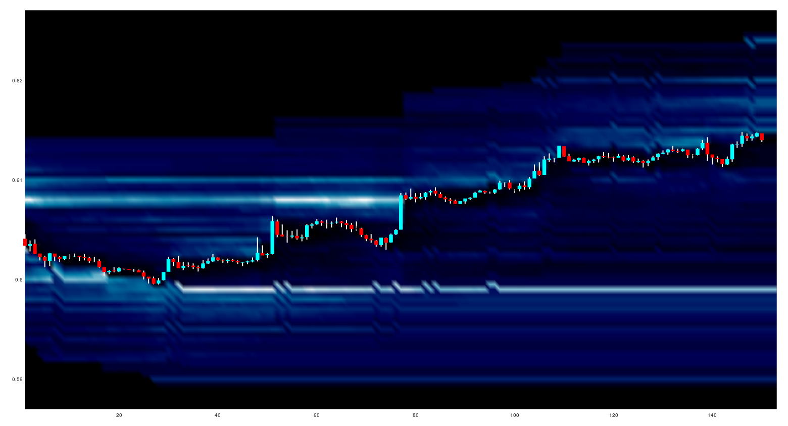
The next little project I have set myself is to do the same as above, but to plot a different version of a market profile chart.
No comments:
Post a Comment