Saturday, 16 May 2020

A Comparison of Charts

Earlier in May I posted about Market Profile with some charts and video. Further work on this has made me realise that my earlier post should more accurately be described as Volume Profile, so apologies to readers for that.

Another, similar type of chart I have seen described as a TPO chart (TPO stands for 'That Price Occurred' or ticked) and it is a simple matter to extend the code in the above linked post to create a TPO chart and below is the Octave function I have written to produce the backgrounds for both types of plot
## Copyright (C) 2020 dekalog
## 
## This program is free software: you can redistribute it and/or modify it
## under the terms of the GNU General Public License as published by
## the Free Software Foundation, either version 3 of the License, or
## (at your option) any later version.
## 
## This program is distributed in the hope that it will be useful, but
## WITHOUT ANY WARRANTY; without even the implied warranty of
## MERCHANTABILITY or FITNESS FOR A PARTICULAR PURPOSE.  See the
## GNU General Public License for more details.
## 
## You should have received a copy of the GNU General Public License
## along with this program.  If not, see
## .

## -*- texinfo -*- 
## @deftypefn {} {@var{background} =} pcolor_background (@var{y_ax}, @var{high}, @var{low}, @var{vol}, @var{tick_size})
##
## Creates a matrix, BACKGOUND, to be used by Market Profile plotting functions,
## which need a colour background matrix to be plotted by pcolor.
## 
## @seealso{}
## @end deftypefn

## Author: dekalog 
## Created: 2020-05-13

function [ vp_background , mp_background ] = pcolor_background ( y_ax , high , low , vol , tick_size )

vp_z = zeros( 1 , numel( y_ax ) ) ; mp_z = vp_z ;
vol( vol <= 1 ) = 2 ; ## no single point vol distributions

for ii = 1 : numel( high )

## the volume profile, vp_background
ticks = norminv( linspace(0,1,vol(ii)+2) , (high(ii) + low(ii))/2 , (high(ii) - low(ii))*0.25 ) ;
ticks = floor( ticks( 2 : end - 1 ) ./ tick_size .+ 0.5 ) .* tick_size ;
unique_ticks = unique( ticks ) ;

if ( numel( unique_ticks ) > 1 )
[ N , X ] = hist( ticks , unique( ticks ) ) ;
[ ~ , N_ix ] = max( N ) ; tick_ix = X( N_ix ) ;
[ ~ , centre_tick ] = min( abs( y_ax .- tick_ix ) ) ;
vp_z(1,centre_tick-N_ix+1:centre_tick+(numel(N)-N_ix)) = vp_z(1,centre_tick-N_ix+1:centre_tick+(numel(N)-N_ix)).+ N ;
elseif ( numel( unique_ticks ) == 1 )
[ ~ , centre_tick ] = min( abs( y_ax .- unique_ticks ) ) ;
vp_z( 1 , centre_tick ) = vp_z( 1 , centre_tick ) + vol( ii ) ;
endif

## the market profile, mp_background
[ ~ , ix_high ] = min( abs( y_ax .- high( ii ) ) ) ;
[ ~ , ix_low ] = min( abs( y_ax .- low( ii ) ) ) ;
mp_z( 1 , ix_low : ix_high ) = mp_z( 1 , ix_low : ix_high ) .+ 1 ;

endfor

vp_background = repmat( vp_z , numel( high ) , 1 ) ;
mp_background = repmat( mp_z , numel( high ) , 1 ) ;

endfunction
I have elected to still call the TPO plot a Market Profile plot as, from what I can make out, the tick count of the TPO is intended to be a surrogate for the original, cleared volume of Market Profile.

The above function is intended to provide a matrix input for the pcolor function, which internally scales the matrix to 0-1. Another idea I have had is to multiply the Volume Profile matrix and the Market Profile matrix together to get a normalised Combined Profile matrix. The animated GIF below shows all three.
It can be seen that there are subtle differences between them but that, on the whole, the results are similar.

More in due course.

Friday, 8 May 2020

A Second Orderbook Visualisation Chart

Below is code for a second way of charting ohlc price with Oanda's order book levels. First, the function loads the relevant data and plots the order book levels with Octave's pcolor function and then plots the price ohlc as candlesticks over the pcolor plot. The candlestick part of the function reuses some of the code I wrote for the financial package's candle plotting function.
## Copyright (C) 2020 dekalog
## 
## This program is free software: you can redistribute it and/or modify it
## under the terms of the GNU General Public License as published by
## the Free Software Foundation, either version 3 of the License, or
## (at your option) any later version.
## 
## This program is distributed in the hope that it will be useful, but
## WITHOUT ANY WARRANTY; without even the implied warranty of
## MERCHANTABILITY or FITNESS FOR A PARTICULAR PURPOSE.  See the
## GNU General Public License for more details.
## 
## You should have received a copy of the GNU General Public License
## along with this program.  If not, see
## .

## -*- texinfo -*- 
## @deftypefn {} candle_with_order_levels (@var{cross}, @var{n_bars})
##
## Plots a 20 minute candlestick chart of the most recent N_BARS of currency CROSS with
## the background highlighted with Oanda's historical orderbook levels for
## this CROSS.
##
## @seealso{candle,snake_and_canyon_plot}
## @end deftypefn

## Author: dekalog 
## Created: 2020-05-06

function candle_with_order_levels ( curr_cross , n_bars )

price_name = tolower( curr_cross ) ;

## get price data of *_ohlc_20m
unix_command = [ "wc" , " " , "-l" , " " , [ price_name , '_ohlc_20m' ] ] ;
## the 'wc' with '-l' flag command counts the number of lines in [ price_name , '_ohlc_20m' ] } 
[ ~ , system_out ] = system( unix_command ) ;
cstr = strsplit( system_out , " " ) ; 
lines_in_file = str2double( cstr( 1 , 1 ) ) ;
## read *_ohlc_20m file
price_data = dlmread( [ price_name , '_ohlc_20m' ] , ',' , [ lines_in_file - n_bars , 0 , lines_in_file , 21 ] ) ;
open = price_data(:,18) ; high = price_data(:,19) ; low = price_data(:,20) ; close = price_data(:,21) ; vol = price_data(:,22) ;

## get orderbook data of *_historical_orderbook_snapshots
unix_command = [ "wc" , " " , "-l" , " " , [ price_name , '_historical_orderbook_snapshots' ] ] ;
## the 'wc' with '-l' flag command counts the number of lines in [ price_name , '_historical_orderbook_snapshots' ] } 
[ ~ , system_out ] = system( unix_command ) ;
cstr = strsplit( system_out , " " ) ; 
lines_in_file = str2double( cstr( 1 , 1 ) ) ;
## read *_ohlc_20m file
orderbook_data = dlmread( [ price_name , '_historical_orderbook_snapshots' ] , ',' , [ lines_in_file - n_bars , 0 , lines_in_file , 87 ] ) ;
## combine buys and sell % and delete unnecessary data
orderbook_data( : , 7 : 47 ) = orderbook_data( : , 7 : 47 ) .+ orderbook_data( : , 48 : 88 ) ;
orderbook_data( : , 48 : 88 ) = [] ; ## col( : , 27 ) is the orderbook price level column

## create the backgound heatmap of levels
if ( strcmp( price_name , 'aud_jpy' ) || strcmp( price_name , 'eur_jpy' ) || strcmp( price_name , 'gbp_jpy' ) || ...
     strcmp( price_name , 'usd_jpy' ) )
 bucket_size = 0.05 ;
elseif ( strcmp( price_name , 'xau_usd' ) )
 bucket_size = 0.5 ;
else
 bucket_size = 0.0005 ;
endif

rounded_order_price = round( orderbook_data( : , 6 ) ./ bucket_size ) .* bucket_size ;

## create and fill image mesh for backgound plot
y_max = max( rounded_order_price .+ ( 20 * bucket_size ) ) ;
y_min = min( rounded_order_price .- ( 20 * bucket_size ) ) ;
y_ax = ( y_min - 5 * bucket_size : bucket_size : y_max + 5 * bucket_size )' ;
x_ax = ( 1 : 1 : numel( open ) + 3 )' ;

z = zeros( numel( x_ax ) , numel( y_ax ) ) ;

##for ii = 1 : size( z , 2 )
##[ ~ , ix ] = min( abs( y_ax .- rounded_order_price( ii ) ) ) ;
##z( ix - 20 : ix + 20 , ii ) = orderbook_data( ii , 7 : 47 )' ;
##endfor

[ ~ , ix ] = min( abs( y_ax .- rounded_order_price( 1 ) ) ) ;
z( 1 , ix - 20 : ix + 20 ) = orderbook_data( 1 , 7 : 47 ) ;
for ii = 2 : numel( x_ax ) - 3
z( ii , : ) = z( ii - 1 , : ) ;
[ ~ , ix ] = min( abs( y_ax .- rounded_order_price( ii ) ) ) ;
z( ii , ix - 20 : ix + 20 ) = orderbook_data( ii , 7 : 47 ) ;
endfor

for ii = numel( x_ax ) - 2 : numel( x_ax )
z( ii , : ) = z( ii - 1 , : ) ;
endfor

## For pcolor(), if x and y are vectors, then a typical vertex is (x(j), y(i), c(i,j)). 
## Thus, columns of c correspond to different x values and rows of c correspond to different y values.
## create the background ( best choices - viridis and ocean? ) 
colormap( 'ocean' ) ; figure( 20 ) ; pcolor( x_ax , y_ax , z' ) ; shading interp ; axis tight ;

hold on ; 

## plot candlesticks
wicks = high .- low ;
body = close .- open ;
up_down = sign ( body );
body_width = 20 ;
wick_width = 2 ;
doji_size = 10 ;
one_price_size = 15 ;

## plot the wicks
x = ( 1 : numel( close ) ) ;  # the x-axis
idx = x ;
high_nan = nan( size ( high ) ) ; high_nan( idx ) = high ; # highs
low_nan = nan( size ( low ) ) ; low_nan( idx ) = low ;     # lows
x = reshape( [ x ; x ; nan( size ( x ) ) ] , [] , 1 ) ;
y = reshape( [ high_nan( : )' ; low_nan( : )' ; nan( 1 , length ( high ) ) ] , [] , 1 ) ;
figure( 20 ) ; plot( x , y , 'w' , 'linewidth' , wick_width ) ; # plot wicks

## plot the up bar bodies
x = ( 1 : numel( close ) ) ; # the x-axis
idx = ( up_down == 1 ) ; idx = find ( idx ) ;                      # index by condition close > open
high_nan = nan( size ( high ) ) ; high_nan( idx ) = close( idx ) ; # body highs
low_nan = nan( size ( low ) ) ; low_nan( idx ) = open( idx ) ;     # body lows
x = reshape( [ x ; x ; nan( size ( x ) ) ] , [] , 1 ) ;
y = reshape( [ high_nan( : )' ; low_nan( : )' ; nan( 1 , length ( high ) ) ] , [] , 1 ) ;
figure( 20 ) ; plot( x , y , 'c' , 'linewidth' , body_width ) ; # plot bodies for up bars

## plot the down bar bodies
x = ( 1 : numel( close ) ) ; # the x-axis
idx = ( up_down == -1 ) ; idx = find ( idx ) ;                    # index by condition close < open
high_nan = nan( size ( high ) ) ; high_nan( idx ) = open( idx ) ; # body highs
low_nan = nan( size ( low ) ) ; low_nan( idx ) = close( idx ) ;   # body lows
x = reshape( [ x ; x ; nan( size ( x ) ) ] , [] , 1 ) ;
y = reshape( [ high_nan( : )' ; low_nan( : )' ; nan( 1 , length ( high ) ) ] , [] , 1 ) ;
figure( 20 ) ; plot( x , y , 'r' , 'linewidth', body_width ) ; # plot bodies for down bars

## plot special cases
## doji bars
doji_bar = ( high > low ) .* ( close == open ) ; doji_ix = find ( doji_bar ) ;

if ( length ( doji_ix ) >= 1 )
  x = ( 1 : length ( close ) ) ; # the x-axis
  figure( 20 ) ; plot( x( doji_ix ) , close( doji_ix ) , '+k' , 'markersize' , doji_size ) ; # plot the open/close as horizontal dash
endif

## open == high == low == close
one_price = ( high == low ) .* ( close == open ) .* ( open == high ) ; one_price_ix = find ( one_price ) ;

if ( length ( one_price_ix ) >= 1 )
  x = ( 1 : numel( close ) ) ; # the x-axis
  figure( 20 ) ; plot ( x( one_price_ix ) , close( one_price_ix ) , '.k' , 'markersize' , one_price_size ) ; # plot as a point/dot
endif

hold off ;

endfunction
The 20 orderbook levels above and below the open of each candlestick are plotted and a typical looking chart output, with the "ocean" colourmap, is:
where the lighter colours show a higher proportion of accumulated orders.

The next little project I have set myself is to do the same as above, but to plot a different version of a market profile chart.

Tuesday, 5 May 2020

Recording Oanda's Streaming Prices

As a quick update following on from my previous post about Market Profile, with a bit of help I have written the following command line code to capture streaming prices to file
stdbuf -oL -eL curl -s -H "Content-Type: application/json" -H "Authorization: Bearer XXX..." "https://stream-fxtrade.oanda.com/v3/accounts/XXX-XXX-XXXXXX-XXX/pricing/stream?instruments=EUR_USD" | jq --raw-output --unbuffered '[.time, .bids[0].price, .asks[0].price] | @csv' | sed -u 's/["Z]//g' | sed -u 's/[-T:]/,/g' >> ~/path/to/append/to/output
In my previous post I mentioned that capturing streaming tick data would be a whole new infrastructure project, however it seems that the above one line of code in the command line would suffice. I still do not intend to routinely capture such streaming tick data for a host of reasons, but I am going to capture some data in order to calibrate the approach used in my previous post.

More in due course. 

Sunday, 3 May 2020

Market Profile Chart in Octave

In a comment on my previous post, visualising Oanda's orderbook, a reader called Darren suggested that I was over complicating things and should perhaps use a more established methodology, namely Market Profile.

I had heard of Market Profile before Darren mentioned it, but had always assumed that it required access to data that I didn't readily have to hand, i.e. tick level data. With my recent work on Oanda's API in Octave that is no longer necessarily the case. However, downloading, storing and manipulating streams of tick data would be a whole new infrastructure project that I would have to implement in either R or Octave.

Instead of doing this I have done some research into Market Profile and come up with an alternative solution that can use the more readily available tick volume. One of the empirically observed assumptions of Market Profile is that on a "normal" day such volume is normally distributed and creates a "value area" that contains approximately 70% of the market action, which roughly corresponds to action falling within one standard deviation of the mean of said action, and this mean in turn roughly corresponds with what is termed the "point of control" (POC).

If one takes this at face value as being an accurate description of market action, it is possible to recreate the "normal" market profile with the following Octave code:
 ticks = norminv( linspace( 0 , 1 , vol( ii ) + 2 ) , ( high( ii ) + low( ii ) ) / 2 , ( high( ii ) - low( ii ) ) / 6 ) ;
 ticks = floor( ticks( 2 : end - 1 ) ./ tick_size .+ tick_size ) .* tick_size ;
 [ vals , bin_centres ] = hist( ticks , unique( ticks ) ) ;
What this does is create vol(ii)+2 linearly spaced tick values from 0 to 1, where vol(ii) is the tick volume for an aggregated period, i.e. an ohlc bar, and transforms these into normally distributed ticks with a mean of the midpoint of the bar and an assumed standard deviation of one sixth the high-low range, rounded to the nearest whole tick. The hist function then provides the counts of ticks per level (vals) at levels (bin_centres).

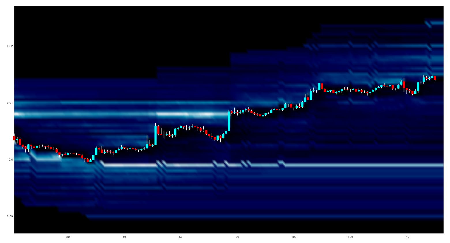
Below is a screen shot of recent EUR_USD forex prices at a resolution of 20 minute candlesticks from 17:00 EST on 28th April 2020 to end of week close at 17:00 EST 1st May 2020.
The silhouette chart at the bottom is the usual tick volume per bar and the horizontal histogram is the Market Profile of the 20 minute bars from the first bar to the first vertical green line, calculated as described above. All the visable vertical green lines represent the open at 07:00 BST, whilst the vertical red lines are the 17:00 EST closes. The horizontal blue line is the current POC at 07:00 BST, taking into account only the bars to the left of the first green line, i.e. the Asian overnight session.

Next is a video of the progression through time along the above chart: as time progesses the Market Profile histogram changes and new, blue POC lines are plotted, with the time progression being marked by the advancing green lines. During subsequent Asian sessions the histogram colour is plotted in red, and new POC lines formed in the Asian session are also plotted in red.


For easier viewing, this is a screen shot of the chart as it appears at the end of the video
For comparative purposes this is a screen shot of the same as above, but using 10 minute ohlc bars and 10 minute updates to the Market Profile
Readers should note that the scaling of the silhouette charts and histograms are not the same for both - they are hand scaled by me for visualisation purposes only.

For completeness, here is the Octave script used to produce the above
clear all ;
pkg load statistics ;

## load data
cd /home/dekalog/Documents/octave/oanda_data/20m ;
oanda_files_20m = glob( "*_ohlc_20m" ) ;
ix = 7 ;##input( 'Tradable? ' ) ;
data = dlmread( oanda_files_20m{ ix } ) ;
data( 1 : 146835 , : ) = [] ;

tick_size = 0.0001 ;

open = data( : , 18 ) ; high = data( : , 19 ) ; low = data( : , 20 ) ; close = data( : , 21 ) ; vol = data( : , 22 ) ;
## Create grid for day
max_high = max( high ) + 0.001 ; min_low = min( low ) - 0.001 ; grid = ( min_low : tick_size : max_high + 0.0001 ) ;
grid_ix = floor( grid ./ tick_size .+ tick_size ) .* tick_size ; 
market_profile = [ grid_ix ; zeros( 1 , size( grid_ix , 2 ) ) ] ;
asian_market_profile = [ grid_ix ; zeros( 1 , size( grid_ix , 2 ) ) ] ;
 
figure( 20 ) ; 
candle( high , low , close , open ) ; 
vline( 27 , 'g' ) ; vline( 72 , 'r' ) ; vline( 99 , 'g' ) ; vline( 144 , 'r' ) ; vline( 174 , 'g' ) ;
xlim( [ 0 size( open , 1 ) ] ) ;
ylim( [ grid_ix(1) grid_ix(end) ] ) ;
hold on ; plot( ( vol .* 0.0000004 ) .+ grid_ix( 1 ) , 'b' , 'linewidth' , 2 ) ; 
area( ( vol .* 0.0000004 ) .+ grid_ix( 1 ) , 'facecolor' , 'b' ) ; hold off ;

for ii = 1 : 27
 ticks = norminv( linspace( 0 , 1 , vol( ii ) + 2 ) , ( high( ii ) + low( ii ) ) / 2 , ( high( ii ) - low( ii ) ) / 6 ) ;
 ticks = floor( ticks( 2 : end - 1 ) ./ tick_size .+ tick_size ) .* tick_size ;
 [ vals , bin_centres ] = hist( ticks , unique( ticks ) ) ;
 vals_ix = find( ismember( grid_ix , bin_centres ) ) ;
 market_profile( 2 , vals_ix ) += vals ;
endfor

[ max_mp_val_old , max_mp_ix ] = max( market_profile( 2 , : ) ) ;

hold on ; figure( 20 ) ; H = barh( market_profile( 1 , : ) , market_profile( 2 , : ).*0.005 , 'c' ) ; hold off ;
hline( market_profile( 1 , max_mp_ix ) , 'b' ) ;

for ii = 28 : 72
 ticks = norminv( linspace( 0 , 1 , vol( ii ) + 2 ) , ( high( ii ) + low( ii ) ) / 2 , ( high( ii ) - low( ii ) ) / 6 ) ;
 ticks = floor( ticks( 2 : end - 1 ) ./ tick_size .+ tick_size ) .* tick_size ;
 vals = hist( ticks , unique( ticks ) ) ;
 vals_ix = find( ismember( grid_ix , unique( ticks ) ) ) ;
 market_profile( 2 , vals_ix ) += vals ;
 [ max_mp_val , max_mp_ix ] = max( market_profile( 2 , : ) ) ;
 hold on ; figure( 20 ) ; barh( market_profile( 1 , : ) , market_profile( 2 , : ).*0.005 , 'c' ) ; hold off ;
 vline( ii , 'g' ) ; 
 if ( max_mp_val > max_mp_val_old )
  hline( market_profile( 1 , max_mp_ix ) , 'b' ) ;
  max_mp_val_old = max_mp_val ;
 endif
 pause(0.01) ;
endfor

for ii = 73 : 99
 ticks = norminv( linspace( 0 , 1 , vol( ii ) + 2 ) , ( high( ii ) + low( ii ) ) / 2 , ( high( ii ) - low( ii ) ) / 6 ) ;
 ticks = floor( ticks( 2 : end - 1 ) ./ tick_size .+ tick_size ) .* tick_size ;
 vals = hist( ticks , unique( ticks ) ) ;
 vals_ix = find( ismember( grid_ix , unique( ticks ) ) ) ;
 market_profile( 2 , vals_ix ) += vals ;
 asian_market_profile( 2 , vals_ix ) += vals ;
 [ max_mp_val , max_mp_ix ] = max( market_profile( 2 , : ) ) ;
 hold on ; figure( 20 ) ; barh( market_profile( 1 , : ) , market_profile( 2 , : ).*0.005 , 'c' ) ; 
 figure( 20 ) ; barh( asian_market_profile( 1 , : ) , asian_market_profile( 2 , : ).*0.005 , 'r' ) ;
 hold off ;
 vline( ii , 'g' ) ; 
 if ( max_mp_val > max_mp_val_old )
  hline( market_profile( 1 , max_mp_ix ) , 'b' ) ;
  max_mp_val_old = max_mp_val ;
 endif
 pause(0.01) ;
endfor

[ ~ , max_mp_ix ] = max( asian_market_profile( 2 , : ) ) ;
hline( asian_market_profile( 1 , max_mp_ix ) , 'r' ) ;

for ii = 100 : 144
 ticks = norminv( linspace( 0 , 1 , vol( ii ) + 2 ) , ( high( ii ) + low( ii ) ) / 2 , ( high( ii ) - low( ii ) ) / 6 ) ;
 ticks = floor( ticks( 2 : end - 1 ) ./ tick_size .+ tick_size ) .* tick_size ;
 vals = hist( ticks , unique( ticks ) ) ;
 vals_ix = find( ismember( grid_ix , unique( ticks ) ) ) ;
 market_profile( 2 , vals_ix ) += vals ;
 [ max_mp_val , max_mp_ix ] = max( market_profile( 2 , : ) ) ;
 hold on ; figure( 20 ) ; barh( market_profile( 1 , : ) , market_profile( 2 , : ).*0.005 , 'c' ) ;
 figure( 20 ) ; barh( asian_market_profile( 1 , : ) , asian_market_profile( 2 , : ).*0.005 , 'r' ) ; 
 hold off ;
 vline( ii , 'g' ) ; 
 if ( max_mp_val > max_mp_val_old )
  hline( market_profile( 1 , max_mp_ix ) , 'b' ) ;
  max_mp_val_old = max_mp_val ;
 endif
 pause(0.01) ;
endfor

[ max_mp_val , max_mp_ix ] = max( market_profile( 2 , 101 : end ) ) ;
max_mp_val_old = max_mp_val ;
hline( market_profile( 1 , max_mp_ix + 100 ) , 'b' ) ;

for ii = 145 : 174
 ticks = norminv( linspace( 0 , 1 , vol( ii ) + 2 ) , ( high( ii ) + low( ii ) ) / 2 , ( high( ii ) - low( ii ) ) / 6 ) ;
 ticks = floor( ticks( 2 : end - 1 ) ./ tick_size .+ tick_size ) .* tick_size ;
 vals = hist( ticks , unique( ticks ) ) ;
 vals_ix = find( ismember( grid_ix , unique( ticks ) ) ) ;
 market_profile( 2 , vals_ix ) += vals ;
 asian_market_profile( 2 , vals_ix ) += vals ;
 [ max_mp_val , max_mp_ix ] = max( market_profile( 2 , 101 : end ) ) ;
 hold on ; figure( 20 ) ; barh( market_profile( 1 , : ) , market_profile( 2 , : ).*0.005 , 'c' ) ; 
 figure( 20 ) ; barh( asian_market_profile( 1 , : ) , asian_market_profile( 2 , : ).*0.005 , 'r' ) ;
 hold off ;
 vline( ii , 'g' ) ; 
 if ( max_mp_val > max_mp_val_old )
  hline( market_profile( 1 , max_mp_ix + 100 ) , 'b' ) ;
  max_mp_val_old = max_mp_val ;
 endif
 pause(0.01) ;
endfor

[ ~ , max_mp_ix ] = max( asian_market_profile( 2 , 101 : end ) ) ;
hline( asian_market_profile( 1 , max_mp_ix + 100 ) , 'r' ) ;

for ii = 175 : size( open , 1 )
 ticks = norminv( linspace( 0 , 1 , vol( ii ) + 2 ) , ( high( ii ) + low( ii ) ) / 2 , ( high( ii ) - low( ii ) ) / 6 ) ;
 ticks = floor( ticks( 2 : end - 1 ) ./ tick_size .+ tick_size ) .* tick_size ;
 vals = hist( ticks , unique( ticks ) ) ;
 vals_ix = find( ismember( grid_ix , unique( ticks ) ) ) ;
 market_profile( 2 , vals_ix ) += vals ;
 [ max_mp_val , max_mp_ix ] = max( market_profile( 2 , 101 : end ) ) ;
 hold on ; figure( 20 ) ; barh( market_profile( 1 , : ) , market_profile( 2 , : ).*0.005 , 'c' ) ; 
 figure( 20 ) ; barh( asian_market_profile( 1 , : ) , asian_market_profile( 2 , : ).*0.005 , 'r' ) ;
 hold off ;
 vline( ii , 'g' ) ; 
 if ( max_mp_val > max_mp_val_old )
  hline( market_profile( 1 , max_mp_ix + 100 ) , 'b' ) ;
  max_mp_val_old = max_mp_val ;
 endif
 pause(0.01) ;
endfor
As just noted above for the scaling of the charts/video, readers should also be aware that within this script there are a lot of magic numbers that are unique to the data and scaling being used; therefore, this is not a plug in and play video script.

My thanks to the reader Darren, who suggested that I look into Market Profile. More in due course.

Thursday, 23 April 2020

Visualising Oanda's Orderbook

My earlier post of 26th March shows code to visualise the most recent instantaneous snapshot of Oanda's order book, realised as a horizontal bar chart superimposed over a price chart. Below is a screen shot of a different type of chart
designed to show the historical order book, which is similar to the proprietary Bookmap software. The background of the chart is a heatmap of the 20 order book levels above and below the order book price, with the lighter colours representing a higher percentage of the total order book order volume, the spheres are sized proportionally to the tick volume of the relevant OHLC bar and the blue and red lines represent the high and low of the bar respectively. The lighter colours nicely highlight the areas where orders are accumulated for potential support and resistance.

However, the above screenshot is actually a two dimensional view, from above, of a three dimensional surface plot, as can be seen in the short video below

The first 25 seconds or so shows panning along the two dimensional view, whilst the remainder of the video shows panning in 3 dimensions. I have whimsically named this a "Snake and Canyon" plot as it resembles watching a river flowing/snaking along a canyon/valley floor and bouncing off the cliffs/hills that are the support and resistance zones. The higher the peaks, the higher the percentage of resting orders, and thus a greater number of incoming market orders is needed to breakout out of the canyon/valley.

I created this so that I can visually look for patterns in the historical data, the reason being that my statistical search for useful features, using the Boruta package, has not shown any useful results yet. The Octave code to produce a "Snake and Canyon" plot is given below. Of course, use of this code presupposes that you have the data available for loading from csv files. Enjoy!
clear all ;
cd /home/dekalog/Documents/octave/oanda_data/20m ;

orderbook_snapshots_files = glob( '*_historical_orderbook_snapshots' ) ;
## {
##   [1,1] = aud_jpy_historical_orderbook_snapshots
##   [2,1] = aud_usd_historical_orderbook_snapshots
##   [3,1] = eur_aud_historical_orderbook_snapshots
##   [4,1] = eur_chf_historical_orderbook_snapshots
##   [5,1] = eur_gbp_historical_orderbook_snapshots
##   [6,1] = eur_jpy_historical_orderbook_snapshots
##   [7,1] = eur_usd_historical_orderbook_snapshots
##   [8,1] = gbp_chf_historical_orderbook_snapshots
##   [9,1] = gbp_jpy_historical_orderbook_snapshots
##   [10,1] = gbp_usd_historical_orderbook_snapshots
##   [11,1] = nzd_usd_historical_orderbook_snapshots
##   [12,1] = usd_cad_historical_orderbook_snapshots
##   [13,1] = usd_chf_historical_orderbook_snapshots
##   [14,1] = usd_jpy_historical_orderbook_snapshots
##   [15,1] = xag_usd_historical_orderbook_snapshots
##   [16,1] = xau_usd_historical_orderbook_snapshots
## }

file_no = input( 'Enter file no. from list, a number 1 to 16 inclusive. ' ) ;
filename = orderbook_snapshots_files{ file_no } ;
str_split = strsplit( filename , "_" ) ;
price_name = strjoin( str_split( 1 : 2 ) , "_" ) ;
ohlc_20m = dlmread( [ price_name , '_ohlc_20m' ] ) ; ## price data
orders = dlmread( [ price_name , '_historical_orderbook_snapshots' ] ) ; ## get latest orderbook levels

if ( file_no == 1 || file_no == 6 || file_no == 9 || file_no == 14 )
 bucket_size = 0.05 ;
elseif ( file_no == 16 )
 bucket_size = 0.5 ;
else
 bucket_size = 0.0005 ;
endif

order_price = orders( : , 6 ) ;
price_length = 250 ;
plot_price = order_price( end - price_length : end ) ;
rounded_price = round( plot_price ./ bucket_size ) .* bucket_size ;
x_length = ( 1 : 1 : ( price_length + 1 ) )' ;

y_max = max( rounded_price .+ ( 20 * bucket_size ) ) ;
y_min = min( rounded_price .- ( 20 * bucket_size ) ) ;
y = ( y_min : bucket_size : y_max )' ;

z = zeros( size( y , 1 ) , size( x_length , 1 ) ) ;
zz = orders( end - price_length : end , 7 : 47 ) .+ orders( end - price_length : end , 48 : 88 ) ;

for ii = 1 : size( z , 2 )
[ ~ , ix ] = min( abs( y .- plot_price( ii ) ) ) ;
z( ix - 20 : ix + 20 , ii ) = zz( ii , : ) ;
endfor

z_high = max( max( z ) ) ;
mid_y = ( ohlc_20m( end - price_length : end , 19 ) .+ ohlc_20m( end - price_length : end , 20 ) ) ./ 2 ;
vol = ohlc_20m( end - price_length : end , 22 ) ; vol = vol ./ max( vol ) ;

up_scatter_ix = find( ohlc_20m( end - price_length : end , 21 ) >= ohlc_20m( end - price_length : end , 18 ) ) ;
down_scatter_ix = find( ohlc_20m( end - price_length : end , 21 ) < ohlc_20m( end - price_length : end , 18 ) ) ;

figure(1) ;
colormap( 'cubehelix' ) ; surf( x_length , y , z , 'edgecolor' , 'none' , 'facecolor' , 'interp' , 'facealpha' , 0.75 ) ; view( 2 ) ; 
axis( [ 1 price_length y_min y_max 0 z_high ] ) ; grid off ;
hold on ;
scatter3( up_scatter_ix , mid_y( up_scatter_ix ) , ones( size( up_scatter_ix ) ) .* z_high ./ 2 , 1000.*vol( up_scatter_ix ) , 'c' , 'o' , 'filled' ) ;
scatter3( down_scatter_ix , mid_y( down_scatter_ix ) , ones( size( down_scatter_ix ) ) .* z_high ./ 2 , 1000.*vol( down_scatter_ix ) , 'm' , 'o' , 'filled' ) ;
line( 'xdata' , x_length , 'ydata' , ohlc_20m( end - price_length : end , 19 ) , 'zdata' , ones(size(x_length)).*z_high ./ 2 , 'color','b' , 'linewidth' , 5 ) ;
line( 'xdata',x_length ,'ydata', ohlc_20m( end - price_length : end , 20 ) ,'zdata', ones(size(x_length)).*z_high ./ 2 , 'color','r' , 'linewidth' , 5 ) ;
xlabel( 'Time' ) ; ylabel( 'Levels - Price' ) ; zlabel( 'OrderBook Percent' ) ; title( strjoin( str_split( 1 : 2 ) , "-" ) ) ;
hold off ;

Wednesday, 15 April 2020

Generic Octave_Oanda_API Function

My last two posts have shown Octave functions that use the Oanda API to access and download data. In the first of these posts I said that I would post more code for further functions as and when I write them. However, on further reflection this would be unnecessary as the generic form of any such function is:

1) create the required headers
## set up the headers
query = [ 'curl -s --compressed -H "Content-Type: application/json"' ] ; ## -s is silent mode for Curl for no paging to terminal
query = [ query , ' -H "Authorization: Bearer XXXXXXXXXXXXXXXXXXXXXXXXXXXXXXXXXXXXXXXXXXXXXXXXXXXXXXXXXXXXXXXXX"' ] ;
2) create the required API call
## construct the actual API call for instrument, year, month, day, hour and min
query = [ query , ' "https://api-fxtrade.oanda.com/v3/instruments/' , toupper( cross ) , "/orderBook?time=" , num2str( year ) , '-' , ...
num2str( month , "%02d" ) , '-' , num2str( day , "%02d" ) , 'T' , num2str( hour , "%02d" ) , '%3A' , num2str( min , "%02d" ) , '%3A00.000Z"' ] ;
3) extract the data from the returned JSON object
## call to use external Unix systems/Curl and return result
[ ~ , ret_JSON ] = system( query , RETURN_OUTPUT = 'TRUE' ) ;

## convert the returned JSON object to Octave structure
ret_JSON = load_json( ret_JSON ) ;
Providing the required libraries are installed on your system (see first post) the above is all that is needed for any API call - just change the details in the second code box - in the example above the code is to download the historical orderbook for a given forex currency cross/tradable at a specific date/time, given as function input variables.

I have found that the main difficulty lies in parsing the returned data structure, which can consist of nested Structures/Cell-Arrays. Below is code, liberally commented, that shows how to parse the above orderbook API call and add the 20 orderbook levels above/below the orderbook price to historical orderbook files already on disc
clear all ;
cd /home/dekalog/Documents/octave/oanda_data/20m ;

orderbooks = glob( '*_historical_orderbook_snapshots' ) ;
## {
##   [1,1] = aud_jpy_historical_orderbook_snapshots
##   [2,1] = aud_usd_historical_orderbook_snapshots
##   [3,1] = eur_aud_historical_orderbook_snapshots
##   [4,1] = eur_chf_historical_orderbook_snapshots
##   [5,1] = eur_gbp_historical_orderbook_snapshots
##   [6,1] = eur_jpy_historical_orderbook_snapshots
##   [7,1] = eur_usd_historical_orderbook_snapshots
##   [8,1] = gbp_chf_historical_orderbook_snapshots
##   [9,1] = gbp_jpy_historical_orderbook_snapshots
##   [10,1] = gbp_usd_historical_orderbook_snapshots
##   [11,1] = nzd_usd_historical_orderbook_snapshots
##   [12,1] = usd_cad_historical_orderbook_snapshots
##   [13,1] = usd_chf_historical_orderbook_snapshots
##   [14,1] = usd_jpy_historical_orderbook_snapshots
##   [15,1] = xag_usd_historical_orderbook_snapshots
##   [16,1] = xau_usd_historical_orderbook_snapshots
## }
data_20m = glob( '*_ohlc_20m' ) ;

for ii = 1 : 1 ## begin the instrument loop

str_split = strsplit( data_20m{ ii } , "_" ) ;
cross = strjoin( str_split( 1 : 2 ) , "_" ) ; ## get the tradable, e.g. 'eur_usd'

## create a unix system command to read the last row of 20 min ohlc of filename
unix_command = [ "tail -1" , " " , data_20m{ ii } ] ; 
[ ~ , data ] = system( unix_command ) ;
data = strsplit( data , { "," , "\n" } ) ; ## gives a cell arrayfun
## covert last date/time to numeric format
data_20m_last = [ str2num(data{1}) , str2num(data{2}) , str2num(data{3}) , str2num(data{4}) ,str2num(data{5}) ] ;

## create a unix system command to read the last row of historical_orderbook_snapshots of filename
unix_command = [ "tail -1" , " " , orderbooks{ ii } ] ; 
[ ~ , data ] = system( unix_command ) ;
data = strsplit( data , { "," , "\n" } ) ; ## gives a cell arrayfun
## covert last date/time to numeric format
data_ordbk_last = [ str2num(data{1}) , str2num(data{2}) , str2num(data{3}) , str2num(data{4}) ,str2num(data{5}) ] ;

time_diff = datenum( data_20m_last ) - datenum( data_ordbk_last ) ;
## only run following code if there is more orderbook data to download to match 20min data already on file
 if ( time_diff > 0 )

 no_rows_diff = ceil( time_diff * 72 ) ; ## there are 72 x 20 minute bars per day
 ## create a unix system command to read the last no_rows_diff of 20 min ohlc of filename
 unix_command = [ "tail -" , num2str( no_rows_diff ) , " " , data_20m{ ii } ] ; 
 [ ~ , data ] = system( unix_command ) ;
 data = strsplit( data , { "," , "\n" } ) ; ## gives a cell arrayfun
 data = data( 1 : size( data , 2 ) - 1 ) ; ## get rid of last empty cell
 data = reshape( data , 22 , no_rows_diff )' ;
 
  for jj = 1 : no_rows_diff
   if ( str2double(data{jj,1})==data_ordbk_last(1) && str2double(data{jj,2})==data_ordbk_last(2) && ...
        str2double(data{jj,3})==data_ordbk_last(3) && str2double(data{jj,4})==data_ordbk_last(4) && ...
        str2double(data{jj,5})==data_ordbk_last(5) )
    begin_ix = jj + 1 ;
    break ;
   endif
  endfor ## end of jj = 1 : no_rows_diff loop

 new_orderbook_data = zeros( no_rows_diff - ( begin_ix - 1 ) , 88 ) ;

 kk = 0 ; ## initialise kk counter to loop over new_orderbook_data rows
  for jj = begin_ix : no_rows_diff ## loop over structure S from begin_ix to no_rows_diff
   kk = kk + 1 ; ## increment counter
   
   ## write dates and times to new_orderbook_data
   new_orderbook_data( kk , 1 ) = str2double( data{ jj , 1 } ) ;
   new_orderbook_data( kk , 2 ) = str2double( data{ jj , 2 } ) ;
   new_orderbook_data( kk , 3 ) = str2double( data{ jj , 3 } ) ;
   new_orderbook_data( kk , 4 ) = str2double( data{ jj , 4 } ) ;
   new_orderbook_data( kk , 5 ) = str2double( data{ jj , 5 } ) ;
   
   ## download the orderbook structure, S
   S = get_historical_orderbook( cross , new_orderbook_data( kk , 1 ) , new_orderbook_data( kk , 2 ) , new_orderbook_data( kk , 3 ) , ...
                                  new_orderbook_data( kk , 4 ) , new_orderbook_data( kk , 5 ) ) ;

   ## write the orderBook Price to new_orderbook_data
   new_orderbook_data( kk , 6 ) = str2double( S.orderBook.price ) ;

    ######## find where str2double( S.orderBook.price ) is within S ########
    for ix = 1 : size( S.orderBook.buckets , 2 )
     if ( str2double( S.orderBook.buckets{ ix }.price ) >= str2double( S.orderBook.price ) )
      mid_ix = ix ;  
      break ;
     endif
    endfor ## end ix loop

    if ( ( str2double( S.orderBook.price ) - str2double( S.orderBook.buckets{ mid_ix - 1 }.price ) ) < ...
         ( str2double( S.orderBook.buckets{ mid_ix }.price ) ) - str2double( S.orderBook.price ) ) ## refine accuracy of mid_ix
      mid_ix = mid_ix - 1 ;
    endif
    ########## index for str2double( S.orderBook.price ) found #############

  ## actual writing to file: +/- 20 lines around mid_ix, the orderbook_price
  orderbook_begin_ix = mid_ix - 20 ; orderbook_end_ix = mid_ix + 20 ;
  
  ## format of file to write is:
  ## year month day hour min orderbook_price long% short%
   xx = 7 ; ## initialise column counter
   for zz = orderbook_begin_ix : orderbook_end_ix
    new_orderbook_data( kk , xx ) = str2double( S.orderBook.buckets{ zz }.longCountPercent ) ;
    new_orderbook_data( kk , xx + 41 ) = str2double( S.orderBook.buckets{ zz }.shortCountPercent ) ;
    xx = xx + 1 ; ## increment column counter
   endfor ## end of zz filling loop
   
  endfor ## end of jj for loop to fill one line of new_orderbook_data

 endif ## end of ( time_diff > 0 ) if statement

dlmwrite( orderbooks{ ii } , new_orderbook_data , '-append' ) ;

endfor ## end of ii instrument for loop

## The downloaded Structure S looks like
## parse the character structure S and write to new_orderbook_data
##  isstruct(S)
##  ans = 1
##  fieldnames(S)
##  ans =
##  {
##    [1,1] = orderBook
##  }
##
##  >> fieldnames(S.orderBook)
##  ans =
##  {
##    [1,1] = instrument
##    [2,1] = time
##    [3,1] = unixTime
##    [4,1] = price
##    [5,1] = bucketWidth
##    [6,1] = buckets
##  }
##
##  S.orderBook.instrument
##  ans = AUD_JPY
##
##  S.orderBook.time
##  ans = 2020-04-05T21:00:00Z
##
##  S.orderBook.unixTime
##  ans = 1586120400
##
##  S.orderBook.price
##  ans = 65.080
##
##  S.orderBook.bucketWidth
##  ans = 0.050
##
##  iscell( S.orderBook.buckets )
##  ans = 1
The code uses loops, which is usually frowned upon in favour of vectorised code, but I am not aware of how to vectorise the parsing of the structure. This code also shows the use of the unix_command to use -tail to read just the last 'n' lines of the files on disc and thus avoid loading complete, and perhaps very large, files.

Saturday, 11 April 2020

Get Latest Pricing Octave_Oanda_API Function

Following on from my my earlier, simple account summary API function, here is a function which downloads the latest pricing information for a given currency cross/tradable
## Copyright (C) 2020 dekalog
## 
## This program is free software: you can redistribute it and/or modify it
## under the terms of the GNU General Public License as published by
## the Free Software Foundation, either version 3 of the License, or
## (at your option) any later version.
## 
## This program is distributed in the hope that it will be useful, but
## WITHOUT ANY WARRANTY; without even the implied warranty of
## MERCHANTABILITY or FITNESS FOR A PARTICULAR PURPOSE.  See the
## GNU General Public License for more details.
## 
## You should have received a copy of the GNU General Public License
## along with this program.  If not, see
## .

## -*- texinfo -*- 
## @deftypefn {} {@var{best_bid}, @var{best_ask} =} get_current_pricing (@var{currency_cross})
##
## Returns the current pricing (best bid and ask prices) for CURRENCY_CROSS given by the Oanda API call,
## for example,
##
## "https://api-fxtrade.oanda.com/v3/accounts//pricing?instruments=EUR_USD"
##
## for CURRENCY_CROSS == 'eur_usd' (input is a character vector)
##
## Internally the function runs system() which calls the Curl
## library for the actual API download. The function is hard coded
## with the account token and account ID.
##
## @seealso{}
## @end deftypefn

## Author: dekalog 
## Created: 2020-04-05

function [ best_bid , best_ask ] = get_current_pricing ( cross )
 
if ( ischar( cross ) == 0 )
   error( 'Input must be a character vector for currency crosss/tradable, e.g. "eur_usd"' ) ;
endif
 
## set up the headers
query = [ 'curl -s -H "Content-Type: application/json"' ] ; ## -s is silent mode for Curl for no paging to terminal
query = [ query , ' -H "Authorization: Bearer 63926d856d2f6d7ed16ff014c8227042-3ceb540b828a7380b02dfdb273e7ab68"' ] ;

## construct the API call
query = [ query , ' "https://api-fxtrade.oanda.com/v3/accounts/001-004-225017-001/pricing?instruments=' ] ;
query = [ query , toupper( cross ) , '"' ] ;

## call to use external Unix systems/Curl and return result
[ ~ , ret_JSON ] = system( query , RETURN_OUTPUT = 'TRUE' ) ;

## convert the returned JSON object to Octave structure
s = load_json( ret_JSON ) ;

best_bid = s.prices{1}.bids{1}.price ;
best_ask = s.prices{1}.asks{1}.price ;

endfunction

## Typically, the retval output structure s will look like this:-
##
## s =
##
##   scalar structure containing the fields:
##
##     time = 2020-04-10T17:42:13.317424312Z
##     prices =
##     {
##       [1,1] =
##
##         scalar structure containing the fields:
##
##           type = PRICE
##           time = 2020-04-10T17:42:09.734257300Z
##           bids =
##           {
##             [1,1] =
##
##               scalar structure containing the fields:
##
##                 price: 1x7 sq_string
##                 liquidity: 1x1 uint32 scalar
##
##             [1,2] =
##
##               scalar structure containing the fields:
##
##                 price: 1x7 sq_string
##                 liquidity: 1x1 uint32 scalar
##
##             [1,3] =
##
##               scalar structure containing the fields:
##
##                 price: 1x7 sq_string
##                 liquidity: 1x1 uint32 scalar
##
##             [1,4] =
##
##               scalar structure containing the fields:
##
##                 price: 1x7 sq_string
##                 liquidity: 1x1 uint32 scalar
##
##           }
##
##           asks =
##           {
##             [1,1] =
##
##               scalar structure containing the fields:
##
##                 price: 1x7 sq_string
##                 liquidity: 1x1 uint32 scalar
##
##             [1,2] =
##
##               scalar structure containing the fields:
##
##                 price: 1x7 sq_string
##                 liquidity: 1x1 uint32 scalar
##
##             [1,3] =
##
##               scalar structure containing the fields:
##
##                 price: 1x7 sq_string
##                 liquidity: 1x1 uint32 scalar
##
##             [1,4] =
##
##               scalar structure containing the fields:
##
##                 price: 1x7 sq_string
##                 liquidity: 1x1 uint32 scalar
##
##           }
##
##           closeoutBid = 1.09358
##           closeoutAsk = 1.09388
##           status = tradeable
##           tradeable = 1
##           unitsAvailable =
##
##             scalar structure containing the fields:
##
##               default: 1x1 scalar struct
##               openOnly: 1x1 scalar struct
##               reduceFirst: 1x1 scalar struct
##               reduceOnly: 1x1 scalar struct
##
##           quoteHomeConversionFactors =
##
##             scalar structure containing the fields:
##
##               positiveUnits: 1x10 sq_string
##               negativeUnits: 1x10 sq_string
##
##           instrument = EUR_USD
##
##     }
##
## where bid and ask fields etc. just give information rather than values.
## Can access values by, e.g. values = s.prices
## to get
##
## b =
## {
##   [1,1] =
##
##     scalar structure containing the fields:
##
##       type = PRICE
##       time = 2020-04-10T17:48:17.265291655Z
##       bids =
##       {
##         [1,1] =
##
##           scalar structure containing the fields:
##
##             price = 1.09352
##             liquidity = 1000000
##
##         [1,2] =
##
##           scalar structure containing the fields:
##
##             price = 1.09351
##             liquidity = 2000000
##
##         [1,3] =
##
##           scalar structure containing the fields:
##
##             price = 1.09350
##             liquidity = 2000000
##
##         [1,4] =
##
##           scalar structure containing the fields:
##
##             price = 1.09348
##             liquidity = 5000000
##
##       }
##
##       asks =
##       {
##         [1,1] =
##
##           scalar structure containing the fields:
##
##             price = 1.09393
##             liquidity = 1000000
##
##         [1,2] =
##
##           scalar structure containing the fields:
##
##             price = 1.09395
##             liquidity = 2000000
##
##         [1,3] =
##
##           scalar structure containing the fields:
##
##             price = 1.09396
##             liquidity = 2000000
##
##         [1,4] =
##
##           scalar structure containing the fields:
##
##             price = 1.09397
##             liquidity = 5000000
##
##       }
##
##       closeoutBid = 1.09348
##       closeoutAsk = 1.09397
##       status = tradeable
##       tradeable = 1
##       unitsAvailable =
##
##         scalar structure containing the fields:
##
##           default =
##
##             scalar structure containing the fields:
##
##               long: 1x6 sq_string
##               short: 1x6 sq_string
##
##           openOnly =
##
##             scalar structure containing the fields:
##
##               long: 1x6 sq_string
##               short: 1x6 sq_string
##
##           reduceFirst =
##
##             scalar structure containing the fields:
##
##               long: 1x6 sq_string
##               short: 1x6 sq_string
##
##           reduceOnly =
##
##             scalar structure containing the fields:
##
##               long: 1x1 sq_string
##               short: 1x1 sq_string
##
##
##       quoteHomeConversionFactors =
##
##         scalar structure containing the fields:
##
##           positiveUnits = 0.80113441
##           negativeUnits = 0.80178317
##
##       instrument = EUR_USD
##
## }
##
## where some of the values are now "viewable" in terminal.
##
## to do this directly do
##
## s.prices{1}.asks{1}.price, which  will give 1.09393
##
## and 
##
## s.prices{1}.asks{1}.liquidity, which will give 1000000
The function returns are the best bid and ask prices; however, it would be a simple enough task for readers to edit the function to get further levels, a la Market depth, liquidity at these levels and some other price metrics. There is a comment section at the end of the function which shows how to do this.

I wrote this function with a view to it perhaps becoming the basis of a client-side, trailing stop functionality. Enjoy!