Update on Currency Strength Smoothing, and a new direction?

Since my last two posts ( currency strength indicator and preliminary tests thereof ) I have been experimenting with different ways of smoothing the indicators without introducing lag, mostly along the lines of using an oscillator leading signal plus various schemes to smooth and compensate for introduced attenuation and making heavy use of my particle swarm optimisation code. Unfortunately I haven't found anything that really works to my satisfaction and so I have decided to forgo any further attempts at this and just use the indicator in its unsmoothed form as neural net input.

In the process of doing the above work I decided that my particle swarm routine wasn't fast enough and I started using the BayesOpt optimisation library, which is written in C++ and has an interface to Octave. Doing this has greatly decreased the time I've had to spend in my various optimisation routines and the framework provided by the BayesOpt library will enable more ambitious optimisations in the future.

Another discovery for me was this Predicting Stock Market Prices with Physical Laws paper, which has some really useful ideas for neural net input features. In particular I think the idea of combining position, velocity and acceleration with the ideas contained in an earlier post of mine on Savitzky Golay filter convolution and using the currency strength indicators as proxies for the arbitrary sine and cosine waves function posited in the paper hold some promise. More in due course.    

Preliminary Tests of Currency Strength Indicator

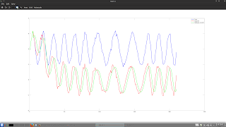
Since my last post on the currency strength indicator I have been conducting a series of basic randomisation tests to see if the indicator has better than random predictive ability. The first test was a random permutation test, as described in Aronson's Evidence Based Technical Analysis book, the code for which I have previously posted on my Data Snooping Tests Github page. These results were all disappointing in that the null hypothesis of no predictive ability cannot be rejected. However, looking at a typical chart ( repeated from the previous post but colour coded for signals )

it can be seen that there are a lot of green ( no signal ) bars which, during the randomisation test, can be selected and give equal or greater returns than the signal bars ( blue for longs, red for shorts ). The relative sparsity of the signal bars compared to non-signal bars gives the permutation test, in this instance, low power to detect significance, although I am not able to show that this is actually true in this case.

In the light of the above I decided to conduct a different test, the .m code for which is shown below.

clear all ;
load all_strengths_quad_smooth_21 ;

all_random_entry_distribution_results = zeros( 21 , 3 ) ;

tic();

for ii = 1 : 21

clear -x ii all_strengths_quad_smooth_21 all_random_entry_distribution_results ;

  if ii == 1
  load audcad_daily_bin_bars ;
  mid_price = ( audcad_daily_bars( : , 3 ) .+ audcad_daily_bars( : , 4 ) ) ./ 2 ; mid_price_rets = [ 0 ; diff( mid_price ) ] ;
  base_ix = 6 ; term_ix = 7 ;
  end
  
  if ii == 2
  load audchf_daily_bin_bars ;
  mid_price = ( audchf_daily_bars( : , 3 ) .+ audchf_daily_bars( : , 4 ) ) ./ 2 ; mid_price_rets = [ 0 ; diff( mid_price ) ] ;
  base_ix = 6 ; term_ix = 4 ;
  end

  if ii == 3
  load audjpy_daily_bin_bars ;
  mid_price = ( audjpy_daily_bars( : , 3 ) .+ audjpy_daily_bars( : , 4 ) ) ./ 2 ; mid_price_rets = [ 0 ; diff( mid_price ) ] ;
  base_ix = 6 ; term_ix = 5 ;
  end
  
  if ii == 4
  load audusd_daily_bin_bars ;
  mid_price = ( audusd_daily_bars( : , 3 ) .+ audusd_daily_bars( : , 4 ) ) ./ 2 ; mid_price_rets = [ 0 ; diff( mid_price ) ] ;
  base_ix = 6 ; term_ix = 1 ;
  end
  
  if ii == 5
  load cadchf_daily_bin_bars ;
  mid_price = ( cadchf_daily_bars( : , 3 ) .+ cadchf_daily_bars( : , 4 ) ) ./ 2 ; mid_price_rets = [ 0 ; diff( mid_price ) ] ;
  base_ix = 7 ; term_ix = 4 ;
  end
  
  if ii == 6
  load cadjpy_daily_bin_bars ;
  mid_price = ( cadjpy_daily_bars( : , 3 ) .+ cadjpy_daily_bars( : , 4 ) ) ./ 2 ; mid_price_rets = [ 0 ; diff( mid_price ) ] ;
  base_ix = 7 ; term_ix = 5 ;
  end
  
  if ii == 7
  load chfjpy_daily_bin_bars ;
  mid_price = ( chfjpy_daily_bars( : , 3 ) .+ chfjpy_daily_bars( : , 4 ) ) ./ 2 ; mid_price_rets = [ 0 ; diff( mid_price ) ] ;
  base_ix = 4 ; term_ix = 5 ;
  end
  
  if ii == 8
  load euraud_daily_bin_bars ;
  mid_price = ( euraud_daily_bars( : , 3 ) .+ euraud_daily_bars( : , 4 ) ) ./ 2 ; mid_price_rets = [ 0 ; diff( mid_price ) ] ;
  base_ix = 2 ; term_ix = 6 ;
  end
  
  if ii == 9
  load eurcad_daily_bin_bars ;
  mid_price = ( eurcad_daily_bars( : , 3 ) .+ eurcad_daily_bars( : , 4 ) ) ./ 2 ; mid_price_rets = [ 0 ; diff( mid_price ) ] ;
  base_ix = 2 ; term_ix = 7 ;
  end
  
  if ii == 10
  load eurchf_daily_bin_bars ;
  mid_price = ( eurchf_daily_bars( : , 3 ) .+ eurchf_daily_bars( : , 4 ) ) ./ 2 ; mid_price_rets = [ 0 ; diff( mid_price ) ] ;
  base_ix = 2 ; term_ix = 4 ;
  end
  
  if ii == 11
  load eurgbp_daily_bin_bars ;
  mid_price = ( eurgbp_daily_bars( : , 3 ) .+ eurgbp_daily_bars( : , 4 ) ) ./ 2 ; mid_price_rets = [ 0 ; diff( mid_price ) ] ;
  base_ix = 2 ; term_ix = 3 ;
  end
  
  if ii == 12
  load eurjpy_daily_bin_bars ;
  mid_price = ( eurjpy_daily_bars( : , 3 ) .+ eurjpy_daily_bars( : , 4 ) ) ./ 2 ; mid_price_rets = [ 0 ; diff( mid_price ) ] ;
  base_ix = 2 ; term_ix = 5 ;
  end
  
  if ii == 13
  load eurusd_daily_bin_bars ;
  mid_price = ( eurusd_daily_bars( : , 3 ) .+ eurusd_daily_bars( : , 4 ) ) ./ 2 ; mid_price_rets = [ 0 ; diff( mid_price ) ] ;
  base_ix = 2 ; term_ix = 1 ;
  end
  
  if ii == 14
  load gbpaud_daily_bin_bars ;
  mid_price = ( gbpaud_daily_bars( : , 3 ) .+ gbpaud_daily_bars( : , 4 ) ) ./ 2 ; mid_price_rets = [ 0 ; diff( mid_price ) ] ;
  base_ix = 3 ; term_ix = 6 ;
  end
  
  if ii == 15
  load gbpcad_daily_bin_bars ;
  mid_price = ( gbpcad_daily_bars( : , 3 ) .+ gbpcad_daily_bars( : , 4 ) ) ./ 2 ; mid_price_rets = [ 0 ; diff( mid_price ) ] ;
  base_ix = 3 ; term_ix = 7 ;
  end
  
  if ii == 16
  load gbpchf_daily_bin_bars ;
  mid_price = ( gbpchf_daily_bars( : , 3 ) .+ gbpchf_daily_bars( : , 4 ) ) ./ 2 ; mid_price_rets = [ 0 ; diff( mid_price ) ] ;
  base_ix = 3 ; term_ix = 4 ;
  end
  
  if ii == 17
  load gbpjpy_daily_bin_bars ;
  mid_price = ( gbpjpy_daily_bars( : , 3 ) .+ gbpjpy_daily_bars( : , 4 ) ) ./ 2 ; mid_price_rets = [ 0 ; diff( mid_price ) ] ;
  base_ix = 3 ; term_ix = 5 ;
  end
  
  if ii == 18
  load gbpusd_daily_bin_bars ;
  mid_price = ( gbpusd_daily_bars( : , 3 ) .+ gbpusd_daily_bars( : , 4 ) ) ./ 2 ; mid_price_rets = [ 0 ; diff( mid_price ) ] ;
  base_ix = 3 ; term_ix = 1 ;
  end
  
  if ii == 19
  load usdcad_daily_bin_bars ;
  mid_price = ( usdcad_daily_bars( : , 3 ) .+ usdcad_daily_bars( : , 4 ) ) ./ 2 ; mid_price_rets = [ 0 ; diff( mid_price ) ] ;
  base_ix = 1 ; term_ix = 7 ;
  end
  
  if ii == 20
  load usdchf_daily_bin_bars ;
  mid_price = ( usdchf_daily_bars( : , 3 ) .+ usdchf_daily_bars( : , 4 ) ) ./ 2 ; mid_price_rets = [ 0 ; diff( mid_price ) ] ;
  base_ix = 1 ; term_ix = 4 ;
  end
  
  if ii == 21
  load usdjpy_daily_bin_bars ;
  mid_price = ( usdjpy_daily_bars( : , 3 ) .+ usdjpy_daily_bars( : , 4 ) ) ./ 2 ; mid_price_rets = [ 0 ; diff( mid_price ) ] ;
  base_ix = 1 ; term_ix = 5 ;
  end
  
  % the returns vectors suitably alligned with position vector
  mid_price_rets = shift( mid_price_rets , -1 ) ;
  sma2 = sma( mid_price_rets , 2 ) ; sma2_rets = shift( sma2 , -2 ) ; sma3 = sma( mid_price_rets , 3 ) ; sma3_rets = shift( sma3 , -3 ) ;
  all_rets = [ mid_price_rets , sma2_rets , sma3_rets ] ;

  % delete burn in and 2016 data ( 2016 reserved for out of sample testing )
  all_rets( 7547 : end , : ) = [] ; all_rets( 1 : 50 , : ) = [] ;

%%%%%%%%%%%%%%%%%%%%%%%%%%%%%%%%%%%%%%%%%%%%%%%%%%%%%%%%%%%%%%%%%%%%%%%%%%%%%%%%%
% simple divergence strategy - be long the uptrending and short the downtrending currency. Uptrends and downtrends determined by crossovers
% of the strengths and their respective smooths
  smooth_base = smooth_2_5( all_strengths_quad_smooth_21(:,base_ix) ) ; smooth_term = smooth_2_5( all_strengths_quad_smooth_21(:,term_ix) ) ;
  test_matrix = ( all_strengths_quad_smooth_21(:,base_ix) > smooth_base ) .* ( all_strengths_quad_smooth_21(:,term_ix) < smooth_term) ; % +1 for longs
  short_vec = ( all_strengths_quad_smooth_21(:,base_ix) < smooth_base ) .* ( all_strengths_quad_smooth_21(:,term_ix) > smooth_term) ; short_vec = find( short_vec ) ;
  test_matrix( short_vec ) = -1 ; % -1 for shorts 
%%%%%%%%%%%%%%%%%%%%%%%%%%%%%%%%%%%%%%%%%%%%%%%%%%%%%%%%%%%%%%%%%%%%%%%%%%%%%%%%%

  % delete burn in and 2016 data
  test_matrix( 7547 : end , : ) = [] ; test_matrix( 1 : 50 , : ) = [] ;
  [ ix , jx , test_matrix_values ] = find( test_matrix ) ;
  no_of_signals = length( test_matrix_values ) ;
 
  % the actual returns performance
  real_results = mean( repmat( test_matrix_values , 1 , size( all_rets , 2 ) ) .* all_rets( ix , : ) ) ;
  
  % set up for randomisation test
  iters = 5000 ;
  imax = size( test_matrix , 1 ) ;
  rand_results_distribution_matrix = zeros( iters , size( real_results , 2 ) ) ;

    for jj = 1 : iters
      rand_idx = randi( imax , no_of_signals , 1 ) ; 
      rand_results_distribution_matrix( jj , : ) = mean( test_matrix_values .* all_rets( rand_idx , : ) ) ;
    endfor
    
  all_random_entry_distribution_results( ii , : ) = ( real_results .- mean( rand_results_distribution_matrix ) ) ./ ...
                                                    ( 2 .* std( rand_results_distribution_matrix ) ) ; 
  
endfor % end of ii loop

toc()

save -ascii all_random_entry_distribution_results all_random_entry_distribution_results ;

plot(all_random_entry_distribution_results(:,1),'k','linewidth',2,all_random_entry_distribution_results(:,2),'b','linewidth',2,...
all_random_entry_distribution_results(:,3),'r','linewidth',2) ; legend('1 day','2 day','3 day');

What the code basically does is construct null hypothesis distributions of 1, 2 and 3 day returns of n random entries, where n is the same number of signal bars -1 or +1 as the currency strength indicator signal. The signal returns are then plotted as a line chart of the distance between random return means and signal return means normalised by 2x the random return standard deviations. In this way values >1 approximately correspond to p values < 0.05. Two typical charts are shown below

The first chart shows the results of the unsmoothed currency strength indicator and the second the smoothed version. From this I surmise that the delay introduced by the smoothing is/will be detrimental to performance and so for the nearest future I shall be working on improving the smoothing algorithm used in the indicator calculations.

Currency Strength Indicator

Over the last few weeks I have been looking into creating a currency strength indicator as input to a Nonlinear autoregressive exogenous model. This has involved a fair bit of online research and I have to say that compared to other technical analysis indicators there seems to be a paucity of pages devoted to the methodology of creating such an indicator. Apart from the above linked Wikipedia page I was only really able to find some discussion threads on some forex forums, mostly devoted to the Metatrader platform, and a few of the more enlightening threads are here, here and here. Another website I found, although not exactly what I was looking for, is marketsmadeclear.com and in particular their Currency Strength Matrix.

In the end I decided to create my own relative currency strength indicator, based on the RSI, by making the length of the indicator adaptive to the measured dominant cycle. The optimal theoretical length for the RSI is half the cycle period, and the price series are smoothed in a [ 1 2 2 1 ] FIR filter prior to the RSI calculations. I used the code in my earlier post to calculate the dominant cycle period, the reason being that since I wrote that post I have watched/listened to a podcast in which John Ehlers recommended using this calculation method for dominant cycle measurement.

The screenshots below are of the currency strength indicator applied to approx. 200 daily bars of the EURUSD forex pair; first the price chart,

next, the indicator,

and finally an oscillator derived from the two separate currency strength lines.

I think the utility of this indicator is quite obvious from these simple charts. Crossovers of the strength lines ( or equivalently, zero line crossings of the oscillator ) clearly indicate major directional changes, and additionally changes in the slope of the oscillator provide an early warning of impending price direction changes.

I will now start to test this indicator and write about these tests and results in due course.

Loading and Manipulating Historical Data From .csv Files

In my last post I said I was going to look at data wrangling my data, and this post outlines what I have done since then.

My problem was that I have numerous csv files containing historical data with different date formats and frequency, e.g. tick level and hourly and daily OHLC, and in the past I have always struggled with this. However, I have finally found a solution using the R quantmod package, which makes it easy to change data into a lower frequency. It took me some time to finally get what I wanted but the code box below shows the relevant R code to convert hourly OHLC, contained in one .csv file, to daily OHLC which is then written to a new .csv file.

library("quantmod", lib.loc="~/R/x86_64-pc-linux-gnu-library/3.3")
price_data = read.csv( "path/to/file.csv" , header = FALSE )
price_data = xts( price_data[,2:6] , order.by = as.Date.POSIXlt( strptime( price_data[,1] , format = "%d/%m/%y %H:%M" , tz = "" ) ) )
price_data_daily = to.daily( price_data , drop.time = TRUE )
write.zoo( price_data_daily , file = "path/to/new/file.csv" , sep = "," , row.names = FALSE , col.names = FALSE )

To finally achieve such a small snippet of working code I can't believe how much time I had to spend reading documentation and looking online.

This next code box shows Octave code to load the above written .csv file into Octave

fid = fopen( 'path/to/file' , 'rt' ) ;
data = textscan( fid , '%s %f %f %f %f' , 'Delimiter' , ',' , 'CollectOutput', 1 ) ;
fclose( fid ) ;
eurusd = [ datenum( data{1} , 'yyyy-mm-dd' ) data{2} ] ;
clear data fid

Hopefully, in both cases, manipulating the format strings "%d/%m/%y %H:%M" and 'yyyy-mm-dd' in these two respective code snippets will save you the hours I spent.

Useful links that helped me are:

• https://stackoverflow.com/questions/1641519/reading-date-and-time-from-csv-file-in-matlab
• http://www.quantmod.com/examples/data/#aggregate

Possible Addition of NARX Network to Conditional Restricted Boltzmann Machine

It has been over three months since my last post, due to working away from home for some of the summer, a summer holiday and moving home. However, during this time I have continued with my online reading and some new thinking about my conditional restricted boltzmann machine based trading system has developed, namely the use of a nonlinear autoregressive exogenous model in the bottom layer gaussian units of the CRBM. Some links to reading on the same are shown below.

• https://www.mathworks.com/help/nnet/ug/design-time-series-narx-feedback-neural-networks.html 
• http://deeplearning.cs.cmu.edu/pdfs/Narx.pdf 
• http://www.wseas.us/e-library/transactions/research/2008/27-464.pdf 
• https://rucore.libraries.rutgers.edu/rutgers-lib/24889/ 
• https://arxiv.org/abs/1607.02093 
• https://hal.archives-ouvertes.fr/hal-00501643/document 
• http://www.theijes.com/papers/v3-i11/Version-1/C0311019026.pdf 
• http://www.sciencedirect.com/science/article/pii/S0925231208003081 

The exogenous time series I am thinking of using, at least for the major forex pairs and perhaps precious metals, oil and US treasuries, is a currency strength indicator based on the US dollar. In order to create the currency strength indicator I will have to delve into some data wrangling with the historical forex data I have, and this will be the subject of my next post.

Giving Up on Recursive Sine Formula for Period Calculation

I have spent the last few weeks trying to get my recursive sine wave formula for period calculations to work, but try as I might I can only get it to do so under ideal theoretical conditions. Once any significant noise, trend or combination thereof is introduced the calculations explode and give meaningless results. In light of this, I am no longer going to continue this work.

Apart from the above work I have also been doing my usual online research and have come across John Ehler's autocorrelation periodogram for period measurement, and below is my Octave C++ .oct implementation of it.

DEFUN_DLD ( autocorrelation_periodogram, args, nargout,
"-*- texinfo -*-\n\
@deftypefn {Function File} {} autocorrelation_periodogram (@var{input_vector})\n\
This function takes an input vector ( price ) and outputs the dominant cycle period,\n\
calculated from the autocorrelation periodogram spectrum.\n\
@end deftypefn" )

{
octave_value_list retval_list ;
int nargin = args.length () ;

// check the input arguments
if ( nargin != 1 ) // there must be a price vector only
   {
   error ("Invalid arguments. Input is a price vector only.") ;
   return retval_list ;
   }

if ( args(0).length () < 4 )
   {
   error ("Invalid argument length. Input is a price vector of length >= 4.") ;
   return retval_list ;
   }

if ( error_state )
   {
   error ("Invalid argument. Input is a price vector of length >= 4.") ;
   return retval_list ;
   }
// end of input checking 

ColumnVector input = args(0).column_vector_value () ;
ColumnVector hp = args(0).column_vector_value () ; hp.fill( 0.0 ) ;
ColumnVector smooth = args(0).column_vector_value () ; smooth.fill( 0.0 ) ;
ColumnVector corr ( 49 ) ; corr.fill( 0.0 ) ;
ColumnVector cosine_part ( 49 ) ; cosine_part.fill( 0.0 ) ;
ColumnVector sine_part ( 49 ) ; sine_part.fill( 0.0 ) ;
ColumnVector sq_sum ( 49 ) ; sq_sum.fill( 0.0 ) ;
ColumnVector R1 ( 49 ) ; R1.fill( 0.0 ) ;
ColumnVector R2 ( 49 ) ; R2.fill( 0.0 ) ;  
ColumnVector pwr ( 49 ) ; pwr.fill( 0.0 ) ;
ColumnVector dominant_cycle = args(0).column_vector_value () ; dominant_cycle.fill( 0.0 ) ;  
   
double avglength = 3.0 ;
double M ;
double X ; double Y ;   
double Sx ; double Sy ; double Sxx ; double Syy ; double Sxy ;
double denom ;
double max_pwr = 0.0 ;
double Spx ; double Sp ;  

// variables for highpass filter, hard coded for a high cutoff period of 48 bars and low cutoff of 10 bars
double high_cutoff = 48.0 ; double low_cutoff = 10.0 ;  
double alpha_1 = ( cos( 0.707 * 2.0 * PI / high_cutoff ) + sin( 0.707 * 2.0 * PI / high_cutoff ) - 1.0 ) / cos( 0.707 * 2.0 * PI / high_cutoff ) ;   
double beta_1 = ( 1.0 - alpha_1 / 2.0 ) * ( 1.0 - alpha_1 / 2.0 ) ;
double beta_2 = 2.0 * ( 1.0 - alpha_1 ) ;
double beta_3 = ( 1.0 - alpha_1 ) * ( 1.0 - alpha_1 ) ;
 
// variables for super smoother
double a1 = exp( -1.414 * PI / low_cutoff ) ;
double b1 = 2.0 * a1 * cos( 1.414 * PI / low_cutoff ) ;
double c2 = b1 ;
double c3 = -a1 * a1 ;
double c1 = 1.0 - c2 - c3 ;
  
// calculate the automatic gain control factor, K
double K = 0.0 ;
double accSlope = -1.5 ; //acceptableSlope = 1.5 dB
double halfLC = low_cutoff / 2.0 ;
double halfHC = high_cutoff / 2.0 ;
double ratio = pow( 10 , accSlope / 20.0 ) ;
  
 if( halfHC - halfLC > 0.0 )
    {
  K = pow( ratio , 1.0 / ( halfHC - halfLC ) ) ;
    }

// loop to initialise hp and smooth
for ( octave_idx_type ii ( 2 ) ; ii < 49 ; ii++ ) // main loop
    {  
    // highpass filter components whose periods are < 48 bars
    hp(ii) = beta_1 * ( input(ii) - 2.0 * input(ii-1) + input(ii-2) ) + beta_2 * hp(ii-1) - beta_3 * hp(ii-2) ;
    
    // smooth with a super smoother filter
    smooth(ii) = c1 * ( hp(ii) + hp(ii-1) ) / 2.0 + c2 * smooth(ii-1) + c3 * smooth(ii-2) ;
    } // end of initial loop

for ( octave_idx_type ii ( 49 ) ; ii < args(0).length () ; ii++ ) // main loop
    {  
    // highpass filter components whose periods are < 48 bars
    hp(ii) = beta_1 * ( input(ii) - 2.0 * input(ii-1) + input(ii-2) ) + beta_2 * hp(ii-1) - beta_3 * hp(ii-2) ;
    
    // smooth with a super smoother filter
    smooth(ii) = c1 * ( hp(ii) + hp(ii-1) ) / 2.0 + c2 * smooth(ii-1) + c3 * smooth(ii-2) ;
      
      // Pearson correlation for each value of lag
      for ( octave_idx_type lag (0) ; lag <= high_cutoff ; lag++ ) 
          {
          // set the averaging length as M
          M = avglength ;
          if ( avglength == 0) 
             {
              M = double( lag ) ; 
             }
             
          Sx = 0.0 ; Sy = 0.0 ; Sxx = 0.0 ; Syy = 0.0 ; Sxy = 0.0 ;
            
            for ( octave_idx_type count (0) ; count < M - 1 ; count++ )
                {
                 X = smooth(ii-count) ; Y = smooth(ii-(lag+count)) ; 
                 Sx += X ; 
                 Sy += Y ;
                 Sxx += X * X ;
                 Sxy += X * Y ;
                 Syy += Y * Y ;
                }
             
            denom = ( M * Sxx - Sx * Sx ) * ( M * Syy - Sy * Sy ) ;    
            if ( denom > 0.0 )
               {
                corr(lag) = ( M * Sxy - Sx * Sy ) / sqrt( denom ) ;  
               }    
            
          } // end of Pearson correlation loop        
/*
    The DFT is accomplished by correlating the autocorrelation at each value of lag with the cosine and sine of each period of interest. 
    The sum of the squares of each of these values represents the relative power at each period.
*/                  
      for ( octave_idx_type period (low_cutoff) ; period <= high_cutoff ; period++ )
          {
           cosine_part( period ) = 0.0 ; sine_part( period ) = 0.0 ;
            
            for ( octave_idx_type N (3) ; N <= high_cutoff ; N++ )
                {
                 cosine_part( period ) += corr( N ) * cos( 2.0 * PI * double( N ) / double( period ) ) ;  
                 sine_part( period ) += corr( N ) * sin( 2.0 * PI * double( N ) / double( period ) ) ; 
                } // end of N loop
                
            sq_sum( period ) = cosine_part( period ) * cosine_part( period ) + sine_part( period ) * sine_part( period ) ;
                
          } // end of first period loop 
 
      // EMA is used to smooth the power measurement at each period          
      for ( octave_idx_type period (low_cutoff) ; period <= high_cutoff ; period++ )
          {
           R2( period ) = R1( period ) ;
           R1( period ) = 0.2 * sq_sum( period ) * sq_sum( period ) + 0.8 * R2( period ) ; 
          } // end of second period loop
      
    // Find maximum power level for normalisation      
    max_pwr = 0.0 ;      
          
      for ( octave_idx_type period (low_cutoff) ; period <= high_cutoff ; period++ )
          {
           if ( R1( period ) > max_pwr )
              {
                max_pwr = K * R1( period ) ;
              }
          } // end of third period loop
    
    // normalisation of power      
      for ( octave_idx_type period (low_cutoff) ; period <= high_cutoff ; period++ )
          {
           pwr( period ) = R1( period ) / max_pwr ;
          } // end of fourth period loop 
      
    // compute the dominant cycle using the centre of gravity of the spectrum
    Spx = 0.0 ; Sp = 0.0 ;
    
      for ( octave_idx_type period (low_cutoff) ; period <= high_cutoff ; period++ )
          {
           if ( pwr( period ) >= 0.5 )
              {
               Spx += double( period ) * pwr( period ) ;
               Sp += pwr( period ) ;  
              }
          } // end of fifth period loop
    
    if ( Sp != 0.0 )
       {
        dominant_cycle(ii) = Spx / Sp ;
       }      
          
    } // end of main loop
    
retval_list( 0 ) = dominant_cycle ;

return retval_list ;

} // end of function 

When applied directly to a theoretical but noisy sine wave series with a trend I find that this autocorrelation method performs better than my current period measurement algo, but on detrended data it is not as good. Since it is trivial to detrend price data, for now I am going to stick with my current method.

Recursive Sine Wave Formula for Period Calculation

Since my last post I have successfully managed to incorporate the deepmat toolbox into my code, so now my RBM pre-training uses Parallel tempering and adaptive learning rates, which is all well and good. The only draw back at the moment is the training time - it takes approximately 3 to 4 minutes per bar to train on a minimal set of 2 features because the toolbox is written in Octave code and uses for loops instead of using vectorisation. Obviously this is something that I would like to optimise, but for the nearest future I now want to concentrate on feature engineering and create a useful set of features for my CRBM.

In the past I have blogged about frequency/period measurement ( e.g. here and here ) and in this post I would like to talk about a possible new way to calculate the dominant cycle period in the data. In a Stackoverflow forum post some time ago I was alerted to a recursive sinewave generator, with code, that shows how to forward generate a sine wave using just the last few values of a sine wave. It struck me that the code can be used, given the last three values of a sine wave, to calculate the period of the sine wave using simple linear regression, and in the code box below I give some Octave code which shows the basic idea.

clear all

% sine wave periods
period = input( 'Enter period: ' )
period2 = input( 'Enter period2: ' )

true_periods = [ ones( 6*period , 1 ) .* period ; ones( 3*period2 , 1 ) .* period2 ; ones( 3*period , 1 ) .* period ] ;

% create sine wave and add some noise
price = awgn( 1 .* ( 2 .+ [ sinewave( 6*period , period )' ; sinewave( 3*period2 , period2 )' ; sinewave( 3*period , period )' ] ) , 100 ) ;

% extract the signal
hp = highpass_filter_basic( price ) ;

% smooth the signal
smooth = smooth_2_5( hp ) ;

Y = smooth .+ shift( smooth , 2 ) ;
X = shift( smooth , 1 ) ;

calculated_periods = zeros( size ( price ) ) ;

% do the linear regression
for ii = 50 : size( price , 1 )
calculated_periods(ii) = ( ( X( ii-4:ii , : )' * X( ii-4:ii , : ) ) \ X( ii-4:ii , : )' ) * Y( ii-4:ii , : ) ;
end

% get the periods from regression calculations
calculated_periods = real( sqrt( ( 8 .- 4 .* calculated_periods ) ./ ( calculated_periods .+ 2 ) ) ) ;
calculated_periods = 360 ./ ( ( calculated_periods .* 180 ) ./ pi ) ;
calculated_periods = ema( calculated_periods , 3 ) ;
calculated_periods = round( calculated_periods ) ;

figure(1) ; plot( price , 'b' , "linewidth" , 2 , hp , 'r' , "linewidth" , 2 , smooth , 'g' , "linewidth" , 2 ) ; legend( 'Price' , 'Highpass' , 'Highpass smooth' ) ;
figure(2) ; plot( true_periods , 'b' , "linewidth" , 2 , calculated_periods , 'r' , "linewidth", 2 ) ; legend( 'True Periods' , 'Calculated Periods' ) ;

The code creates a sine wave with two periods ( user defined ), does the calculations and then plots the  sine wave and the periods in figures 1 and 2 respectively. The linear regression part of the code use the most recent five bars for calculation, which could of course also be user defined. On data without added noise typical plots are :-

which shows the underlying "price" in blue and the high pass filtered and smoothed versions in red and green and

shows the true and measured periods. Noisy price versions of the above are :-

and

Theoretically it seems to work, but I would like to see if things can be improved. More in my next post.