Brownian Bands revisited?

Further to my most recent post there have been a few anonymous comments suggesting that Brownian bands are more useful than I supposed. In response I have added a contact form to this blog ( on the right ) so these anonymous readers may contact me if they wish. I am curious to learn how they may be using Brownian bands. I might also add that I have thought of creating a new indicator ( a kind of randomness measurement oscillator ) based on the Brownian bands concept.

Suspending Work on Brownian Bands

Recently I have been doing a lot of work looking at various uses of the Brownian bands but I have been unable to come up with anything unique that I feel can help me so for now I am going to discontinue this work. There may be a time in the future when I return to this, but for now the Brownian bands are going to be put on the shelf along with my other indicators.

I have also started to become disillusioned with my attempts at creating a market classifier neural net; I think it may very well be too large a project to complete satisfactorily, so I am going to try something simpler in concept at least. In large part this change of heart is due to some recent reading I have been doing, particularly this article in which I was struck by the phrase

"As an aside, the ideal "trades" formed by the turning points might make a good training set of trades for a neural network-based system. Rather than scanning a chart manually to come up with trades to feed into the neural network, the method described here could be used to automatically find the training set."

Also over on the Mechanical Forex site there is a whole series of articles on neural nets which I have found useful and have given me a new insight. I am now going to ask readers to suspend their disbelief for a few moments while I explain.

Imagine it is a few minutes before the trading open and you have to decide whether to enter long, short or remain out of the market when the market opens. However, unlike any other market participant, the Gods have given you a gift - the ability to see the near future - which means you know the OHLC for today, tomorrow and the next trading day. But, as with all gifts from the Gods, there is a catch - you can only enter and exit trades at the market open; there is no buying the low and selling the high of a candlestick bar or intraday trading permitted by the Gods. What would such a blessed but responsible trader do? How would they make their trade decision? Being responsible s/he might consider the reward to risk ratio and only take a trade if this ratio is greater than one: on the long side the maximum open of tomorrow or the day after minus today's open divided by today's open minus the minimum low of today, tomorrow or the day after: and a similar reasoning for the short side. If neither of these ratios is greater than one, no new trade will be entered today.

The upper pane in the video below shows the coding of such logic. The decision to go long is rendered in blue, short in red and neutral in green. The colour of the bar indicates the action to be taken at the open of the next bar. However, it might be that when a neutral signal is given there is already be a position held, in which case the existing position is held for the duration of the neutral signal. This is effectively an always in the market, stop and reverse signal, and this is shown in the lower pane of the video. To make things slightly easier to see the entry/exit action occurs at the open of a new colour bar, i.e. if the bars change from blue to red the long is exited and the short initiated at the open of the first red bar.

Non-embedded view.  

Even with a cursory viewing it can be seen what a great "system" this would be, and using neural nets to create such a "system" is now my ambition.

The plan is simple: roll a moving window along the price series and use the known relationships between bars and indicators within this window to train a locally optimised neural net. The purpose of the training will be to classify the bars as long entry, short entry or neutral as in the chart in the upper pane of the above video. At the hard right edge of the chart the last three bars will be unavailable to the neural net for training purposes, but the hope is that the neural net, sufficiently well trained on all data in the window immediately prior to these three bars, will have predictive ability for them. After all, in the main, market dynamics slowly evolve over a few bars rather than dramatically leap.

Before I embark on this new work there are a few optimisation tests I would like to conduct, and these tests will form the subject matter of my next few posts.

Brownian Bands

For the past few weeks I have been working on the idea presented in my earlier modelling prices using brownian motion post and below is a video of what I have come up with, which I'm calling Brownian Bands. The video shows these bands on the EURUSD forex pair with look back lengths of 1 to 10 bars inclusive, then 15 to 50 in increments of 5, then 50, 100 and 200 and finally 50, 100 and 200 on the whole time series. Each look back length band is the average of all bands from 1 up to and including the look back length band - the details of the implementation can be seen in the code boxes below. The blue band is the upper band, the red is the lower and the green is the mid point of the two.

           
Non-embedded view.

This following chart shows an adaptive look back length implementation, the look back length being determined by a period vector input to the function, which in this case is the dominant cycle period.

These adaptive Brownian bands can be compared with the equivalent adaptive Bollinger bands shown in this next chart.

For my intended purpose of separating out returns into distribution bins the Brownian bands seem to be superior. There are 3 distinct bins: above the upper band, below the lower band and between the bands, whereas with the Bollinger bands the vast majority of returns would be lumped into just one bin - between the bands. Of course the Brownian bands could be used to create a system indicator just as Bollinger bands can be, and if any readers test this idea I would be intrigued to hear of your results. However, should you choose to do this there is a major caveat you should be aware of. The calculation of the Brownian bands is based on the natural log of actual price, which means you should be very wary of test results on any back adjusted price series such as futures and adjusted stock prices. In fact I would go as far to say that the code given below should not be used as is on such price series. It is for this reason that I have been using forex price series in my own tests so far, but I will surely get around to adjusting the given code in due course.

Now for the code. This first code box shows a hard-coded, unrolled loop version for look back lengths up to and including 25 for the benefit of a reader who requested a clearer exposition of the method than was given in my earlier post, which was vectorised Octave code. All the code below is C++ as used in Octave .oct files.

DEFUN_DLD ( brownian_bands_25, args, nargout, 
"-*- texinfo -*-\n\
@deftypefn {Function File} {} brownian_bands_25 (@var{price,period})\n\
This function takes a price vector input and a value for the tick\n\
size of the instrument and outputs upper and lower bands based on\n\
the concept of Brownian motion. The bands are the average of look\n\
back periods of 1 to 25 bars inclusive of the relevant calculations.\n\
@end deftypefn" )

{
octave_value_list retval_list ;
int nargin = args.length () ;

// check the input arguments
if ( nargin != 2 )
   {
   error ( "Invalid arguments. Type help to see usage." ) ;
   return retval_list ;
   }

if ( args(0).length () < 21 )
   {
   error ( "Invalid arguments. Type help to see usage." ) ;
   return retval_list ;
   }
   
if ( args(1).length () != 1 )
   {
   error ( "Invalid arguments. Type help to see usage." ) ;
   return retval_list ;
   }   

if ( error_state )
   {
   error ( "Invalid arguments. Type help to see usage." ) ;
   return retval_list ;
   }
// end of input checking   

ColumnVector price = args(0).column_vector_value () ;
double tick_size = args(1).double_value() ;
ColumnVector abs_log_price_diff = args(0).column_vector_value () ;
ColumnVector upper_band = args(0).column_vector_value () ;
ColumnVector lower_band = args(0).column_vector_value () ;
ColumnVector mid_band = args(0).column_vector_value () ;
double sum ;

double up_1 ;
double low_1 ;

double up_2 ;
double low_2 ;
double sqrt_2 = sqrt(2.0) ; // pre-calculated for speed optimisation

double up_3 ;
double low_3 ;
double sqrt_3 = sqrt(3.0) ; // pre-calculated for speed optimisation

double up_4 ;
double low_4 ;
double sqrt_4 = sqrt(4.0) ; // pre-calculated for speed optimisation

double up_5 ;
double low_5 ;
double sqrt_5 = sqrt(5.0) ; // pre-calculated for speed optimisation

double up_6 ;
double low_6 ;
double sqrt_6 = sqrt(6.0) ; // pre-calculated for speed optimisation

double up_7 ;
double low_7 ;
double sqrt_7 = sqrt(7.0) ; // pre-calculated for speed optimisation

double up_8 ;
double low_8 ;
double sqrt_8 = sqrt(8.0) ; // pre-calculated for speed optimisation

double up_9 ;
double low_9 ;
double sqrt_9 = sqrt(9.0) ; // pre-calculated for speed optimisation

double up_10 ;
double low_10 ;
double sqrt_10 = sqrt(10.0) ; // pre-calculated for speed optimisation

double up_11 ;
double low_11 ;
double sqrt_11 = sqrt(11.0) ; // pre-calculated for speed optimisation

double up_12 ;
double low_12 ;
double sqrt_12 = sqrt(12.0) ; // pre-calculated for speed optimisation

double up_13 ;
double low_13 ;
double sqrt_13 = sqrt(13.0) ; // pre-calculated for speed optimisation

double up_14 ;
double low_14 ;
double sqrt_14 = sqrt(14.0) ; // pre-calculated for speed optimisation

double up_15 ;
double low_15 ;
double sqrt_15 = sqrt(15.0) ; // pre-calculated for speed optimisation

double up_16 ;
double low_16 ;
double sqrt_16 = sqrt(16.0) ; // pre-calculated for speed optimisation

double up_17 ;
double low_17 ;
double sqrt_17 = sqrt(17.0) ; // pre-calculated for speed optimisation

double up_18 ;
double low_18 ;
double sqrt_18 = sqrt(18.0) ; // pre-calculated for speed optimisation

double up_19 ;
double low_19 ;
double sqrt_19 = sqrt(19.0) ; // pre-calculated for speed optimisation

double up_20 ;
double low_20 ;
double sqrt_20 = sqrt(20.0) ; // pre-calculated for speed optimisation

double up_21 ;
double low_21 ;
double sqrt_21 = sqrt(21.0) ; // pre-calculated for speed optimisation

double up_22 ;
double low_22 ;
double sqrt_22 = sqrt(22.0) ; // pre-calculated for speed optimisation

double up_23 ;
double low_23 ;
double sqrt_23 = sqrt(23.0) ; // pre-calculated for speed optimisation

double up_24 ;
double low_24 ;
double sqrt_24 = sqrt(24.0) ; // pre-calculated for speed optimisation

double up_25 ;
double low_25 ;
double sqrt_25 = sqrt(25.0) ; // pre-calculated for speed optimisation

for ( octave_idx_type ii (1) ; ii < 25 ; ii++ ) // initialising loop 
    {
    abs_log_price_diff(ii) = fabs( log( price(ii) ) - log( price(ii-1) ) ) ;
    }
    
for ( octave_idx_type ii (25) ; ii < args(0).length () ; ii++ ) // main loop
    {
      
    abs_log_price_diff(ii) = fabs( log( price(ii) ) - log( price(ii-1) ) ) ;

    sum = abs_log_price_diff(ii) ;
    up_1 = exp( log( price(ii-1) ) + sum ) ;
    low_1 = exp( log( price(ii-1) ) - sum ) ;

    sum += abs_log_price_diff(ii-1) ;
    up_2 = exp( log( price(ii-2) ) + (sum/2.0) * sqrt_2 ) ;
    low_2 = exp( log( price(ii-2) ) - (sum/2.0) * sqrt_2 ) ;

    sum += abs_log_price_diff(ii-2) ;
    up_3 = exp( log( price(ii-3) ) + (sum/3.0) * sqrt_3 ) ;
    low_3 = exp( log( price(ii-3) ) - (sum/3.0) * sqrt_3 ) ;
    
    sum += abs_log_price_diff(ii-3) ;
    up_4 = exp( log( price(ii-4) ) + (sum/4.0) * sqrt_4 ) ;
    low_4 = exp( log( price(ii-4) ) - (sum/4.0) * sqrt_4 ) ;

    sum += abs_log_price_diff(ii-4) ;
    up_5 = exp( log( price(ii-5) ) + (sum/5.0) * sqrt_5 ) ;
    low_5 = exp( log( price(ii-5) ) - (sum/5.0) * sqrt_5 ) ;    

    sum += abs_log_price_diff(ii-5) ;
    up_6 = exp( log( price(ii-6) ) + (sum/6.0) * sqrt_6 ) ;
    low_6 = exp( log( price(ii-6) ) - (sum/6.0) * sqrt_6 ) ;
    
    sum += abs_log_price_diff(ii-6) ;
    up_7 = exp( log( price(ii-7) ) + (sum/7.0) * sqrt_7 ) ;
    low_7 = exp( log( price(ii-7) ) - (sum/7.0) * sqrt_7 ) ;
    
    sum += abs_log_price_diff(ii-7) ;
    up_8 = exp( log( price(ii-8) ) + (sum/8.0) * sqrt_8 ) ;
    low_8 = exp( log( price(ii-8) ) - (sum/8.0) * sqrt_8 ) ;
    
    sum += abs_log_price_diff(ii-8) ;
    up_9 = exp( log( price(ii-9) ) + (sum/9.0) * sqrt_9 ) ;
    low_9 = exp( log( price(ii-9) ) - (sum/9.0) * sqrt_9 ) ;
    
    sum += abs_log_price_diff(ii-9) ;
    up_10 = exp( log( price(ii-10) ) + (sum/10.0) * sqrt_10 ) ;
    low_10 = exp( log( price(ii-10) ) - (sum/10.0) * sqrt_10 ) ;
    
    sum += abs_log_price_diff(ii-10) ;
    up_11 = exp( log( price(ii-11) ) + (sum/11.0) * sqrt_11 ) ;
    low_11 = exp( log( price(ii-11) ) - (sum/11.0) * sqrt_11 ) ;
    
    sum += abs_log_price_diff(ii-11) ;
    up_12 = exp( log( price(ii-12) ) + (sum/12.0) * sqrt_12 ) ;
    low_12 = exp( log( price(ii-12) ) - (sum/12.0) * sqrt_12 ) ;
    
    sum += abs_log_price_diff(ii-12) ;
    up_13 = exp( log( price(ii-13) ) + (sum/13.0) * sqrt_13 ) ;
    low_13 = exp( log( price(ii-13) ) - (sum/13.0) * sqrt_13 ) ;
    
    sum += abs_log_price_diff(ii-13) ;
    up_14 = exp( log( price(ii-14) ) + (sum/14.0) * sqrt_14 ) ;
    low_14 = exp( log( price(ii-14) ) - (sum/14.0) * sqrt_14 ) ;
    
    sum += abs_log_price_diff(ii-14) ;
    up_15 = exp( log( price(ii-15) ) + (sum/15.0) * sqrt_15 ) ;
    low_15 = exp( log( price(ii-15) ) - (sum/15.0) * sqrt_15 ) ;
    
    sum += abs_log_price_diff(ii-15) ;
    up_16 = exp( log( price(ii-16) ) + (sum/16.0) * sqrt_16 ) ;
    low_16 = exp( log( price(ii-16) ) - (sum/16.0) * sqrt_16 ) ;
    
    sum += abs_log_price_diff(ii-16) ;
    up_17 = exp( log( price(ii-17) ) + (sum/17.0) * sqrt_17 ) ;
    low_17 = exp( log( price(ii-17) ) - (sum/17.0) * sqrt_17 ) ;
    
    sum += abs_log_price_diff(ii-17) ;
    up_18 = exp( log( price(ii-18) ) + (sum/18.0) * sqrt_18 ) ;
    low_18 = exp( log( price(ii-18) ) - (sum/18.0) * sqrt_18 ) ;
    
    sum += abs_log_price_diff(ii-18) ;
    up_19 = exp( log( price(ii-19) ) + (sum/19.0) * sqrt_19 ) ;
    low_19 = exp( log( price(ii-19) ) - (sum/19.0) * sqrt_19 ) ;
    
    sum += abs_log_price_diff(ii-19) ;
    up_20 = exp( log( price(ii-20) ) + (sum/20.0) * sqrt_20 ) ;
    low_20 = exp( log( price(ii-20) ) - (sum/20.0) * sqrt_20 ) ;
    
    sum += abs_log_price_diff(ii-20) ;
    up_21 = exp( log( price(ii-21) ) + (sum/21.0) * sqrt_21 ) ;
    low_21 = exp( log( price(ii-21) ) - (sum/21.0) * sqrt_21 ) ;
    
    sum += abs_log_price_diff(ii-21) ;
    up_22 = exp( log( price(ii-22) ) + (sum/22.0) * sqrt_22 ) ;
    low_22 = exp( log( price(ii-22) ) - (sum/22.0) * sqrt_22 ) ;
    
    sum += abs_log_price_diff(ii-22) ;
    up_23 = exp( log( price(ii-23) ) + (sum/23.0) * sqrt_23 ) ;
    low_23 = exp( log( price(ii-23) ) - (sum/23.0) * sqrt_23 ) ;
    
    sum += abs_log_price_diff(ii-23) ;
    up_24 = exp( log( price(ii-24) ) + (sum/24.0) * sqrt_24 ) ;
    low_24 = exp( log( price(ii-24) ) - (sum/24.0) * sqrt_24 ) ;
    
    sum += abs_log_price_diff(ii-24) ;
    up_25 = exp( log( price(ii-25) ) + (sum/25.0) * sqrt_25 ) ;
    low_25 = exp( log( price(ii-25) ) - (sum/25.0) * sqrt_25 ) ;
    
    upper_band(ii) = (up_1+up_2+up_3+up_4+up_5+up_6+up_7+up_8+up_9+up_10+up_11+up_12+up_13+up_14+up_15+up_16+up_17+up_18+up_19+up_20+up_21+up_22+up_23+up_24+up_25)/25.0 ;
    lower_band(ii) = (low_1+low_2+low_3+low_4+low_5+low_6+low_7+low_8+low_9+low_10+low_11+low_12+low_13+low_14+low_15+low_16+low_17+low_18+low_19+low_20+low_21+low_22+low_23+up_24+low_25)/25.0 ;
    
    // round the upper_band up to the nearest tick
    upper_band(ii) = ceil( upper_band(ii)/tick_size ) * tick_size ;
    
    // round the lower_band down to the nearest tick
    lower_band(ii) = floor( lower_band(ii)/tick_size ) * tick_size ;
    
    mid_band(ii) = ( upper_band(ii) + lower_band(ii) ) / 2.0 ;
    
    } // end of main loop   

    retval_list(2) = mid_band ;
    retval_list(1) = lower_band ;
    retval_list(0) = upper_band ;

return retval_list ;

} // end of function

This next code box contains code for an adjustable look back length, the length being a user input to the function. This code wraps the above unrolled loop into a nested loop.

DEFUN_DLD ( brownian_bands_adjustable, args, nargout, 
"-*- texinfo -*-\n\
@deftypefn {Function File} {} brownian_bands_adjustable (@var{price,lookback,tick_size})\n\
This function takes a price vector input, a value for the lookback\n\
length and a value for the tick size of the instrument and outputs\n\
upper and lower bands based on the concept of Brownian motion. The bands\n\
are the average of lookback period bands from 1 to lookback length.\n\
@end deftypefn" )

{
octave_value_list retval_list ;
int nargin = args.length () ;

// check the input arguments
if ( nargin != 3 )
   {
   error ( "Invalid arguments. Type help to see usage." ) ;
   return retval_list ;
   }
   
if ( args(1).length () != 1 ) // lookback length argument
   {
   error ( "Invalid arguments. Type help to see usage." ) ;
   return retval_list ;
   }
   
double lookback = args(1).double_value() ;   

if ( args(0).length () < lookback ) // check length of price vector input
   {
   error ( "Invalid arguments. Type help to see usage." ) ;
   return retval_list ;
   }
   
if ( args(2).length () != 1 ) // tick size
   {
   error ( "Invalid arguments. Type help to see usage." ) ;
   return retval_list ;
   }   
   
if ( error_state )
   {
   error ( "Invalid arguments. Type help to see usage." ) ;
   return retval_list ;
   }
// end of input checking   

ColumnVector price = args(0).column_vector_value () ;
double tick_size = args(2).double_value() ;
ColumnVector abs_log_price_diff = args(0).column_vector_value () ;
ColumnVector upper_band = args(0).column_vector_value () ;
ColumnVector lower_band = args(0).column_vector_value () ;
ColumnVector mid_band = args(0).column_vector_value () ;
double sum ;
double up_bb ;
double low_bb ;
int jj ;

for ( octave_idx_type ii (1) ; ii < lookback ; ii++ ) // initialising loop 
    {
    abs_log_price_diff(ii) = fabs( log( price(ii) ) - log( price(ii-1) ) ) ;
    }
    
for ( octave_idx_type ii (lookback) ; ii < args(0).length () ; ii++ ) // main loop
    {    
    // initialise calculation values  
    sum = 0.0 ;
    up_bb = 0.0 ;
    low_bb = 0.0 ;

    for ( jj = 1 ; jj < lookback + 1 ; jj++ ) // nested jj loop
        {
   
 abs_log_price_diff(ii) = fabs( log( price(ii) ) - log( price(ii-1) ) ) ;
        sum += abs_log_price_diff(ii-jj+1) ;
        up_bb += exp( log( price(ii-jj) ) + (sum/double(jj)) * sqrt(double(jj)) ) ;
        low_bb += exp( log( price(ii-jj) ) - (sum/double(jj)) * sqrt(double(jj)) ) ;  

 } // end of nested jj loop  
    
    upper_band(ii) = up_bb / lookback ;
    lower_band(ii) = low_bb / lookback ;
    
    // round the upper_band up to the nearest tick
    upper_band(ii) = ceil( upper_band(ii)/tick_size ) * tick_size ;
    
    // round the lower_band down to the nearest tick
    lower_band(ii) = floor( lower_band(ii)/tick_size ) * tick_size ;
    
    mid_band(ii) = ( upper_band(ii) + lower_band(ii) ) / 2.0 ;
    
    } // end of main loop   

    retval_list(2) = mid_band ;
    retval_list(1) = lower_band ;
    retval_list(0) = upper_band ;

return retval_list ;

} // end of function

Finally, this code is the adaptive look back version where the length of the look back is contained in a vector which is also a user input.

DEFUN_DLD ( brownian_bands_adaptive, args, nargout, 
"-*- texinfo -*-\n\
@deftypefn {Function File} {} brownian_bands_adaptive (@var{price,period,tick_size})\n\
This function takes price and period vector inputs & a value for the tick\n\
size of the instrument and outputs upper and lower bands based on\n\
the concept of Brownian motion. The bands are adaptive averages of look\n\
back lengths of 1 to period bars inclusive.\n\
@end deftypefn" )

{
octave_value_list retval_list ;
int nargin = args.length () ;

// check the input arguments
if ( nargin != 3 )
   {
   error ( "Invalid arguments. Type help to see usage." ) ;
   return retval_list ;
   }
   
if ( args(0).length () < 50 ) // check length of price vector input
   {
   error ( "Invalid arguments. Type help to see usage." ) ;
   return retval_list ;
   }   
   
if ( args(1).length () != args(0).length () ) // lookback period length argument
   {
   error ( "Invalid arguments. Type help to see usage." ) ;
   return retval_list ;
   }
      
if ( args(2).length () != 1 ) // tick size
   {
   error ( "Invalid arguments. Type help to see usage." ) ;
   return retval_list ;
   }   
   
if ( error_state )
   {
   error ( "Invalid arguments. Type help to see usage." ) ;
   return retval_list ;
   }
// end of input checking   

ColumnVector price = args(0).column_vector_value () ;
ColumnVector period = args(1).column_vector_value () ; 
double tick_size = args(2).double_value() ;
ColumnVector abs_log_price_diff = args(0).column_vector_value () ;
ColumnVector upper_band = args(0).column_vector_value () ;
ColumnVector lower_band = args(0).column_vector_value () ;
ColumnVector mid_band = args(0).column_vector_value () ;
double sum ;
double up_bb ;
double low_bb ;
int jj ;

for ( octave_idx_type ii (1) ; ii < 50 ; ii++ ) // initialising loop 
    {
    abs_log_price_diff(ii) = fabs( log( price(ii) ) - log( price(ii-1) ) ) ;
    }
    
for ( octave_idx_type ii (50) ; ii < args(0).length () ; ii++ ) // main loop
    {    
    // initialise calculation values  
    sum = 0.0 ;
    up_bb = 0.0 ;
    low_bb = 0.0 ;

    for ( jj = 1 ; jj < period(ii) + 1 ; jj++ ) // nested jj loop
        {
   
 abs_log_price_diff(ii) = fabs( log( price(ii) ) - log( price(ii-1) ) ) ;
        sum += abs_log_price_diff(ii-jj+1) ;
        up_bb += exp( log( price(ii-jj) ) + (sum/double(jj)) * sqrt(double(jj)) ) ;
        low_bb += exp( log( price(ii-jj) ) - (sum/double(jj)) * sqrt(double(jj)) ) ;  

 } // end of nested jj loop  
    
    upper_band(ii) = up_bb / period(ii) ;
    lower_band(ii) = low_bb / period(ii) ;
    
    // round the upper_band up to the nearest tick
    upper_band(ii) = ceil( upper_band(ii)/tick_size ) * tick_size ;
    
    // round the lower_band down to the nearest tick
    lower_band(ii) = floor( lower_band(ii)/tick_size ) * tick_size ;
    
    mid_band(ii) = ( upper_band(ii) + lower_band(ii) ) / 2.0 ;
    
    } // end of main loop   

    retval_list(2) = mid_band ;
    retval_list(1) = lower_band ;
    retval_list(0) = upper_band ;

return retval_list ;

} // end of function

Due to formatting issues on Blogger none of the code boxes contain the required header statements, which should be:-

#include octave/oct.h
#include octave/dColVector.h
#include math.h

with the customary < before "octave" and "math" and > after ".h"

Exploratory Data Analysis of Brownian Motion Model

For my first steps in investigating the earlier proposed Brownian motion model I thought I would use some Exploratory Data Analysis techniques. I have initially decided to use look back periods of 5 bars and 21 bars; the 5 bar on daily data being a crude attempt to capture the essence of weekly price movement and the 21 bar to capture the majority of dominant cycle periods in daily data, with both parameters also being non optimised Fibonacci numbers. Using the two channels over price bars that these create it is possible to postulate nine separate and distinct price "regimes" using combinations of the criteria of being above, within or below each channel.

The use of these "regimes" is to bin normalised price change at time t into nine separate distributions, the normalising factor being the 5 bar simple moving average of absolute natural log differences at time t-1 and the choice of regime being determined by the position of the close at t-1. The rationale behind basing these metrics on preceding bars is explained in this earlier post and the implementation made clear in the code box at the end of this post. The following 4 charts are Box plots of these nine distributions, in consecutive order, for the EURUSD, GBPUSD, USDCHF and USDYEN  forex pairs:

Looking at these, I'm struck by two things. Firstly, the middle three box plots are for regimes where price is in the 21 bar channel, and numbering from the left, boxes 4, 5 and 6 are below the 5 bar channel, in it and above it. These are essentially different degrees of a sideways market and it can be seen that there are far more outliers here than in the other box plots, perhaps indicating the tendency for high volatility breakouts to occur more frequently in sideways markets.

The second thing that is striking is, again numbering from the left, box plots 3 and 7. These are regimes below the 21 bar and above the 5 bar; and above the 21 bar and below the 5 bar - essentially the distributions for reactions against prevailing trends on the 21 bar time scale. Here it can be seen that there are far fewer outliers and generally shorter whiskers, indicating the tendency for reactions against trends to be less volatile in nature.

It is encouraging to see that there are such differences in these box plots as it suggests that my idea of binning does separate out the different price change characteristics. However, I believe things can be improved a bit in this regard and this will form the subject matter of my next post.

clear all

data = load("-ascii","usdyen") ;
close = data(:,7) ;
logdiff = [ 0 ; diff( log(close) ) ] ;
abslogdiff = abs( logdiff ) ;

sq_rt = sqrt( 5 ) ;
sma5 = sma(abslogdiff,5) ;
ub5 = exp(shift(log(close),5).+(sma5.*sq_rt)) ;
lb5 = exp(shift(log(close),5).-(sma5.*sq_rt)) ;

sq_rt = sqrt( 21 ) ;
sma21 = sma(abslogdiff,21) ;
ub21 = exp(shift(log(close),21).+(sma21.*sq_rt)) ;
lb21 = exp(shift(log(close),21).-(sma21.*sq_rt)) ;

% allocate close bar to a market_type
market_type = zeros( size(close,1) , 1 ) ;

% above ub21 **********************
val_1 = close > ub21 ;
val_2 = close > ub5 ;
matches = val_1 .* val_2 ;
ix = find( matches == 1 ) ;
market_type( ix , 1 ) = 4 ;

val_1 = close > ub21 ;
val_2 = close <= ub5 ;
val_3 = close >= lb5 ;
matches = val_1 .* val_2 .* val_3 ;
ix = find( matches == 1 ) ;
market_type( ix , 1 ) = 3 ;

val_1 = close > ub21 ;
val_2 = close < lb5 ;
matches = val_1 .* val_2 ;
ix = find( matches == 1 ) ;
market_type( ix , 1 ) = 2 ;
%**********************************

% below lb21 **********************
val_1 = close < lb21 ;
val_2 = close < lb5 ;
matches = val_1 .* val_2 ;
ix = find( matches == 1 ) ;
market_type( ix , 1 ) = -4 ;

val_1 = close < lb21 ;
val_2 = close <= ub5 ;
val_3 = close >= lb5 ;
matches = val_1 .* val_2 .* val_3 ;
ix = find( matches == 1 ) ;
market_type( ix , 1 ) = -3 ;

val_1 = close < lb21 ;
val_2 = close > ub5 ;
matches = val_1 .* val_2 ;
ix = find( matches == 1 ) ;
market_type( ix , 1 ) = -2 ;
%**********************************

% between ub21 & lb21**************
val_1 = close <= ub21 ;
val_2 = close >= lb21 ;
val_3 = close > ub5 ;
matches = val_1 .* val_2 .* val_3 ;
ix = find( matches == 1 ) ;
market_type( ix , 1 ) = 1 ;

val_1 = close <= ub21 ;
val_2 = close >= lb21 ;
val_3 = close < lb5 ;
matches = val_1 .* val_2 .* val_3 ;
ix = find( matches == 1 ) ;
market_type( ix , 1 ) = -1 ;
%**********************************

% now allocate to bins
normalised_logdiffs = logdiff ./ shift( sma5 , 1 ) ;

% shift market_type to agree with normalised_logdiffs
shifted_market_type = shift( market_type , 1 ) ;

bin_4 = normalised_logdiffs( find( shifted_market_type(30:end,1) == 4 ) , 1 ) ;
bin_3 = normalised_logdiffs( find( shifted_market_type(30:end,1) == 3 ) , 1 ) ;
bin_2 = normalised_logdiffs( find( shifted_market_type(30:end,1) == 2 ) , 1 ) ;
bin_1 = normalised_logdiffs( find( shifted_market_type(30:end,1) == 1 ) , 1 ) ;
bin_0 = normalised_logdiffs( find( shifted_market_type(30:end,1) == 0 ) , 1 ) ;
bin_1m = normalised_logdiffs( find( shifted_market_type(30:end,1) == -1 ) , 1 ) ;
bin_2m = normalised_logdiffs( find( shifted_market_type(30:end,1) == -2 ) , 1 ) ;
bin_3m = normalised_logdiffs( find( shifted_market_type(30:end,1) == -3 ) , 1 ) ;
bin_4m = normalised_logdiffs( find( shifted_market_type(30:end,1) == -4 ) , 1 ) ;

y_axis_max = max( normalised_logdiffs(30:end,1) ) ;
y_axis_min = min( normalised_logdiffs(30:end,1) ) ;

clf ;
subplot(191) ; boxplot(bin_4m,NOTCHED=1) ; ylim([y_axis_min y_axis_max]) ;
subplot(192) ; boxplot(bin_3m,NOTCHED=1) ; ylim([y_axis_min y_axis_max]) ;
subplot(193) ; boxplot(bin_2m,NOTCHED=1) ; ylim([y_axis_min y_axis_max]) ;
subplot(194) ; boxplot(bin_1m,NOTCHED=1) ; ylim([y_axis_min y_axis_max]) ;
subplot(195) ; boxplot(bin_0,NOTCHED=1) ; ylim([y_axis_min y_axis_max]) ;
subplot(196) ; boxplot(bin_1,NOTCHED=1) ; ylim([y_axis_min y_axis_max]) ;
subplot(197) ; boxplot(bin_2,NOTCHED=1) ; ylim([y_axis_min y_axis_max]) ;
subplot(198) ; boxplot(bin_3,NOTCHED=1) ; ylim([y_axis_min y_axis_max]) ;
subplot(199) ; boxplot(bin_4,NOTCHED=1) ; ylim([y_axis_min y_axis_max]) ;

Modelling Prices Using Brownian Motion.

As stated in my previous post I'm going to rewrite my data generation code for future use in online training of neural nets, and the approach I'm going to take is to combine the concept of Brownian motion and the ideas contained in my earlier Creation of Synthetic Data post.

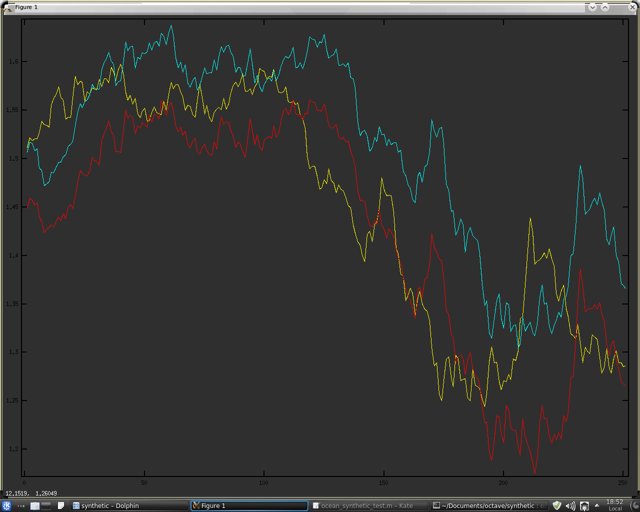
The basic premise, taken from Brownian motion, is that the natural log of price changes, on average, at a rate proportional to the square root of time. Take, for example, a period of 5 leading up to the "current bar." If we take a 5 period simple moving average of the absolute differences of the log of prices over this period, we get a value for the average 1 bar price movement over this period. This value is then multiplied by the square root of 5 and added to and subtracted from the price 5 days ago to get an upper and lower bound for the current bar. If the current bar lies between the bounds, we say that price movement over the last 5 periods is consistent with Brownian motion and declare an absence of trend, i.e. a sideways market. If the current bar lies outside the bounds, we declare that price movement over the last 5 bars is not consistent with Brownian motion and that a trend is in force, either up or down depending on which bound the current bar is beyond. The following 3 charts show this concept in action, for consecutive periods of 5, 13 and 21, taken from the Fibonacci Sequence:

where yellow is the closing price, blue is the upper bound and red the lower bound. It is easy to imagine many uses for this in terms of indicator creation, but I intend to use the bounds to assign a score of price randomness/trendiness over various combined periods to assign price movement to bins for subsequent Monte Carlo creation of synthetic price series. Interested readers are invited to read the above linked Creation of Synthetic Data post for a review of this methodology.

The rough working Octave code that produced the above charts is given below.

clear all

data = load("-ascii","eurusd") ;
% length = input( 'Enter length of look back for calculations: ' ) ;
% sq_rt = sqrt( length ) ;
close = data(:,7) ;
abslogdiff = abs( [ 0 ; diff( log(close) ) ] ) ;

lngth = 3 ;
sq_rt = sqrt( lngth ) ;
sma3 = sma(abslogdiff,lngth) ;
ub = exp(shift(log(close),lngth).+(sma3.*sq_rt)) ;
lb = exp(shift(log(close),lngth).-(sma3.*sq_rt)) ;

all_ub = ub ;
all_lb = lb ;

lngth = 5 ;
sq_rt = sqrt( lngth ) ;
sma5 = sma(abslogdiff,5) ;
ub = exp(shift(log(close),lngth).+(sma5.*sq_rt)) ;
lb = exp(shift(log(close),lngth).-(sma5.*sq_rt)) ;

all_ub = all_ub .+ ub ;
all_lb = all_lb .+ lb ;

lngth = 8 ;
sq_rt = sqrt( lngth ) ;
sma8 = sma(abslogdiff,lngth) ;
ub = exp(shift(log(close),lngth).+(sma8.*sq_rt)) ;
lb = exp(shift(log(close),lngth).-(sma8.*sq_rt)) ;

all_ub = all_ub .+ ub ;
all_lb = all_lb .+ lb ;

lngth = 13 ;
sq_rt = sqrt( lngth ) ;
sma13 = sma(abslogdiff,lngth) ;
ub = exp(shift(log(close),lngth).+(sma13.*sq_rt)) ;
lb = exp(shift(log(close),lngth).-(sma13.*sq_rt)) ;

all_ub = all_ub .+ ub ;
all_lb = all_lb .+ lb ;

lngth = 21 ;
sq_rt = sqrt( lngth ) ;
sma21 = sma(abslogdiff,lngth) ;
ub = exp(shift(log(close),lngth).+(sma21.*sq_rt)) ;
lb = exp(shift(log(close),lngth).-(sma21.*sq_rt)) ;

all_ub = ( all_ub .+ ub ) ./ 5 ;
all_lb = ( all_lb .+ lb ) ./ 5 ;

 plot(close(1850:2100,1),'y',ub(1850:2100,1),'c',lb(1850:2100,1),'r')
%plot(close,'y',ub,'c',lb,'r')

Change of Direction in Neural Net Training.

Up till now when training my neural net classifier I have been using what I call my "idealised" data, which is essentially a model for prices comprised of a sine wave along with a linear trend. In my recent work on Savitzky-Golay filters I wanted to increase the amount of available training data but have run into a problem - the size of my data files has become so large that I'm exhausting the memory available to me in my Octave software install. To overcome this problem I have decided to convert my NN training to an online regime rather than loading csv data files for mini-batch gradient descent training - in fact what I envisage doing would perhaps be best described as online mini-batch training.

To do this will require a fairly major rewrite of my data generation code and I think I will take the opportunity to make this data generation more realistic than the sine wave and trend model I am currently using. Apart from the above mentioned memory problem, this decision has been prompted by an e-mail exchange I have recently had with a reader of this blog and some online reading I have recently been doing, such as mixed regime simulation, training a simple neural network to recognise different regimes in financial time series, neural networks in trading, random subspace optimisation and profitable hidden and markovian coupling. At the moment it is my intention to revisit my earlier posts here and here and use/extend the ideas contained therein. This means that for the nearest future my work on Savitzky-Golay filters is temporarily halted.

Code refactoring didn't work.

In my previous post I said that I was going to refactor code to use my existing, trained classification neural net with Savitzky-Golay filter inputs in the hope that this might show some improvement. I have to report that this was an abysmal failure and I suppose it was a bit naive to have ever expected that it would work. It looks like I will have to explicitly train a new neural network to take advantage of Savitzky-Golay filter features.