Tweaking the Neural Net Inputs

In an attempt to improve my NN system I have recently been thinking of some possibly useful tweaks to the data destined to be the input for the system. Long time readers of this blog will know that the NN system has been trained on my "idealised" data, a typical example of which might look like the red "price series" in the chart below.

These "idealised" series are modelled as simple combinations of linear trend plus a dominant cycle, represented above by the green sine wave at the bottom of the chart. For NN training purposes a mass of training data was created by phase shifting the sine wave and altering the linear trend. However, real data is much more like the cyan "price series," which is modelled as a combination of the linear trend, the dominant or "major" green cycle and a "minor" cyan cycle. It would be possible to create additional NN training data by creating numerous training series comprised of two cycles plus trend, but due to the curse of dimensionality that way madness lies, in addition to the inordinate amount of time it would take to train the NNs.

So the problem becomes one of finding a principled method of transforming the cyan "real data" to be more like the "idealised" red data my NNs were trained on, and a possible answer might be the use of my bandpass indicator. Shown below is a chart of said bandpass indicator overlaid on the above chart, in yellow. The bandpass is set to pass only the "minor" cycle and then this is subtracted from the "real data" to give an

approximation of the red "idealised" data. This particular instance calculates the bandpass with a moving window with a look back length set to the period of the "minor" cycle, whilst the following is a fully recursive implementation. It can be seen that this

recursive implementation is much better on this contrived toy example. However, I think this method shows promise and I intend to pursue it further. More in due course.

Random Permutation of Price Series

As a prelude to the tests mentioned in my previous post it has been necessary to write code to randomly permute price data, and in the code box below is the Octave .oct file I have written to do this.

#include octave oct.h
#include octave dcolvector.h
#include math.h
#include algorithm
#include "MersenneTwister.h"

DEFUN_DLD (randomised_price_data, args, , "Inputs are OHLC column vectors and tick size. Output is permuted synthetic OHLC")
{
octave_value_list retval_list ;
int nargin = args.length () ;
int vec_length = args(0).length () - 1 ;

    if ( nargin != 5 )
    {
        error ("Invalid arguments. Inputs are OHLC column vectors and tick size.") ;
        return retval_list ;
    }

    if (args(0).length () < 50)
    {
        error ("Invalid arguments. Inputs are OHLC column vectors and tick size.") ;
        return retval_list ;
    }

    if (error_state)
    {
        error ("Invalid arguments. Inputs are OHLC column vectors and tick size.") ;
        return retval_list ;
    }

    ColumnVector open = args(0).column_vector_value () ; // open vector
    ColumnVector high = args(1).column_vector_value () ; // high vector
    ColumnVector low = args(2).column_vector_value () ; // low vector
    ColumnVector close = args(3).column_vector_value () ; // close vector
    double tick = args(4).double_value(); // Tick size

    //double trend_increment = ( close ( args(3).length () - 1 ) - close (0) ) / ( args(3).length () - 1 ) ; 
    
    ColumnVector open_change_var ( vec_length ) ;
    ColumnVector high_change_var ( vec_length ) ;
    ColumnVector low_change_var ( vec_length ) ;
    ColumnVector close_change_var ( vec_length ) ;

    // variables for shuffling
    double temp ; 
    int k1 ;
    int k2 ;
    
    // Check for negative or zero price values due to continuous back- adjusting of price series & compensate if necessary
    // Note: the "&" below acts as Address-of operator: p = &x; Read: Assign to p (a pointer) the address of x.
    double lowest_low = *std::min_element( &low(0), &low(low.length()) ) ;
    double correction_factor = 0.0 ;
    if ( lowest_low <= 0.0 )
    {
    correction_factor = fabs(lowest_low) + tick;
 for (octave_idx_type ii (0); ii < args(0).length (); ii++)
 {
 open (ii) = open (ii) + correction_factor;
 high (ii) = high (ii) + correction_factor;
 low (ii) = low (ii) + correction_factor;
 close (ii) = close (ii) + correction_factor;
 }
    }

    // fill the change vectors with their values
    for ( octave_idx_type ii (1) ; ii < args(0).length () ; ii++ )
    {
    // comment out/uncomment depending on whether to include a relationship to previous bar's volatility or not 
    
    // No relationship
    // open_change_var (ii-1) = log10( open (ii) / close (ii) ) ;
    // high_change_var (ii-1) = log10( high (ii) / close (ii) ) ;
    // low_change_var (ii-1) = log10( low (ii) / close (ii) ) ;
    
    // some relationship
    open_change_var (ii-1) = ( close (ii) - open (ii) ) / ( high (ii-1) - low (ii-1) ) ;
    high_change_var (ii-1) = ( close (ii) - high (ii) ) / ( high (ii-1) - low (ii-1) ) ;
    low_change_var (ii-1) = ( close (ii) - low (ii) ) / ( high (ii-1) - low (ii-1) ) ;
    close_change_var (ii-1) = log10( close(ii) / close(ii-1) ) ;
    }
    
 // Shuffle the log vectors

 MTRand mtrand1 ; // Declare the Mersenne Twister Class - will seed from system time
 
       k1 = vec_length - 1 ; // initialise prior to shuffling

       while ( k1 > 0 ) // While at least 2 left to shuffle
             {          
             k2 = mtrand1.randInt( k1 ) ; // Pick an int from 0 through k1 

               if ( k2 > k1 ) // check if random vector index no. k2 is > than max vector index - should never happen 
                  {
                  k2 = k1 - 1 ; // But this is cheap insurance against disaster if it does happen
                  }

             temp = open_change_var (k1) ; // allocate the last vector index content to temp
             open_change_var (k1) = open_change_var (k2) ; // allocate random pick to the last vector index
             open_change_var (k2) = temp ; // allocate temp content to old vector index position of random pick
             
             temp = high_change_var (k1) ; // allocate the last vector index content to temp
             high_change_var (k1) = high_change_var (k2) ; // allocate random pick to the last vector index
             high (k2) = temp ; // allocate temp content to old vector index position of random pick
             
             temp = low_change_var (k1) ; // allocate the last vector index content to temp
             low_change_var (k1) = low_change_var (k2) ; // allocate random pick to the last vector index
             low_change_var (k2) = temp ; // allocate temp content to old vector index position of random pick
             
             temp = close_change_var (k1) ; // allocate the last vector index content to temp
             close_change_var (k1) = close_change_var (k2) ; // allocate random pick to the last vector index
             close_change_var (k2) = temp ; // allocate temp content to old vector index position of random pick
             
             k1 = k1 - 1 ; // count down 
             } // Shuffling is complete when this while loop exits
     
    // create the new shuffled price series and round to nearest tick
    for ( octave_idx_type ii (1) ; ii < args(0).length () ; ii++ )
    { 
    close (ii) = ( floor( ( close (ii-1) * pow( 10, close_change_var(ii-1) ) ) / tick + 0.5 ) ) * tick ;
    
    // comment out/uncomment depending on whether to include a relationship to previous bar's volatility or not
    
    // no relationship
    // open (ii) = ( floor( ( close (ii) * pow( 10, open_change_var(ii-1) ) ) / tick + 0.5 ) ) * tick ;
    // high (ii) = ( floor( ( close (ii) * pow( 10, high_change_var(ii-1) ) ) / tick + 0.5 ) ) * tick ;
    // low (ii) = ( floor( ( close (ii) * pow( 10, low_change_var(ii-1) ) ) / tick + 0.5 ) ) * tick ;
    
    // some relationship
    open (ii) = ( floor( ( open_change_var(ii-1) * ( high (ii-1) - low (ii-1) ) + close (ii) ) / tick + 0.5 ) ) * tick ;
    high (ii) = ( floor( ( high_change_var(ii-1) * ( high (ii-1) - low (ii-1) ) + close (ii) ) / tick + 0.5 ) ) * tick ;
    low (ii) = ( floor( ( low_change_var(ii-1) * ( high (ii-1) - low (ii-1) ) + close (ii) ) / tick + 0.5 ) ) * tick ;
    } 
    
    // if compensation due to negative or zero original price values due to continuous back- adjusting of price series took place, re-adjust
    if ( correction_factor != 0.0 )
    {
 for ( octave_idx_type ii (0); ii < args(0).length () ; ii++ )
 {
 open (ii) = open (ii) - correction_factor ;
 high (ii) = high (ii) - correction_factor ;
 low (ii) = low (ii) - correction_factor ;
 close (ii) = close (ii) - correction_factor ;
 }
    }

retval_list (3) = close ;
retval_list (2) = low ;    
retval_list (1) = high ;
retval_list (0) = open ;

return retval_list ;

} // end of function

The function can be compiled in two slightly different versions by commenting/commenting out some indicated code:- this makes it possible to choose between having more or less dependency between adjacent bars based on the range of the first bar. For completeness the required header file for the Mersenne Twister algorithm is given next

// MersenneTwister.h
// Mersenne Twister random number generator -- a C++ class MTRand
// Based on code by Makoto Matsumoto, Takuji Nishimura, and Shawn Cokus
// Richard J. Wagner  v1.1  28 September 2009  wagnerr@umich.edu

// The Mersenne Twister is an algorithm for generating random numbers.  It
// was designed with consideration of the flaws in various other generators.
// The period, 2^19937-1, and the order of equidistribution, 623 dimensions,
// are far greater.  The generator is also fast; it avoids multiplication and
// division, and it benefits from caches and pipelines.  For more information
// see the inventors' web page at
// http://www.math.sci.hiroshima-u.ac.jp/~m-mat/MT/emt.html

// Reference
// M. Matsumoto and T. Nishimura, "Mersenne Twister: A 623-Dimensionally
// Equidistributed Uniform Pseudo-Random Number Generator", ACM Transactions on
// Modeling and Computer Simulation, Vol. 8, No. 1, January 1998, pp 3-30.

// Copyright (C) 1997 - 2002, Makoto Matsumoto and Takuji Nishimura,
// Copyright (C) 2000 - 2009, Richard J. Wagner
// All rights reserved.
// 
// Redistribution and use in source and binary forms, with or without
// modification, are permitted provided that the following conditions
// are met:
// 
//   1. Redistributions of source code must retain the above copyright
//      notice, this list of conditions and the following disclaimer.
//
//   2. Redistributions in binary form must reproduce the above copyright
//      notice, this list of conditions and the following disclaimer in the
//      documentation and/or other materials provided with the distribution.
//
//   3. The names of its contributors may not be used to endorse or promote 
//      products derived from this software without specific prior written 
//      permission.
// 
// THIS SOFTWARE IS PROVIDED BY THE COPYRIGHT HOLDERS AND CONTRIBUTORS "AS IS"
// AND ANY EXPRESS OR IMPLIED WARRANTIES, INCLUDING, BUT NOT LIMITED TO, THE
// IMPLIED WARRANTIES OF MERCHANTABILITY AND FITNESS FOR A PARTICULAR PURPOSE
// ARE DISCLAIMED.  IN NO EVENT SHALL THE COPYRIGHT OWNER OR CONTRIBUTORS BE
// LIABLE FOR ANY DIRECT, INDIRECT, INCIDENTAL, SPECIAL, EXEMPLARY, OR
// CONSEQUENTIAL DAMAGES (INCLUDING, BUT NOT LIMITED TO, PROCUREMENT OF
// SUBSTITUTE GOODS OR SERVICES; LOSS OF USE, DATA, OR PROFITS; OR BUSINESS
// INTERRUPTION) HOWEVER CAUSED AND ON ANY THEORY OF LIABILITY, WHETHER IN
// CONTRACT, STRICT LIABILITY, OR TORT (INCLUDING NEGLIGENCE OR OTHERWISE)
// ARISING IN ANY WAY OUT OF THE USE OF THIS SOFTWARE, EVEN IF ADVISED OF THE
// POSSIBILITY OF SUCH DAMAGE.

// The original code included the following notice:
// 
//     When you use this, send an email to: m-mat@math.sci.hiroshima-u.ac.jp
//     with an appropriate reference to your work.
// 
// It would be nice to CC: wagnerr@umich.edu and Cokus@math.washington.edu
// when you write.

#ifndef MERSENNETWISTER_H
#define MERSENNETWISTER_H

// Not thread safe (unless auto-initialization is avoided and each thread has
// its own MTRand object)

#include 
#include 
#include 
#include 
#include 

class MTRand {
// Data
public:
 typedef unsigned long uint32;  // unsigned integer type, at least 32 bits
 
 enum { N = 624 };       // length of state vector
 enum { SAVE = N + 1 };  // length of array for save()

protected:
 enum { M = 397 };  // period parameter
 
 uint32 state[N];   // internal state
 uint32 *pNext;     // next value to get from state
 int left;          // number of values left before reload needed

// Methods
public:
 MTRand( const uint32 oneSeed );  // initialize with a simple uint32
 MTRand( uint32 *const bigSeed, uint32 const seedLength = N );  // or array
 MTRand();  // auto-initialize with /dev/urandom or time() and clock()
 MTRand( const MTRand& o );  // copy
 
 // Do NOT use for CRYPTOGRAPHY without securely hashing several returned
 // values together, otherwise the generator state can be learned after
 // reading 624 consecutive values.
 
 // Access to 32-bit random numbers
 uint32 randInt();                     // integer in [0,2^32-1]
 uint32 randInt( const uint32 n );     // integer in [0,n] for n < 2^32
 double rand();                        // real number in [0,1]
 double rand( const double n );        // real number in [0,n]
 double randExc();                     // real number in [0,1)
 double randExc( const double n );     // real number in [0,n)
 double randDblExc();                  // real number in (0,1)
 double randDblExc( const double n );  // real number in (0,n)
 double operator()();                  // same as rand()
 
 // Access to 53-bit random numbers (capacity of IEEE double precision)
 double rand53();  // real number in [0,1)
 
 // Access to nonuniform random number distributions
 double randNorm( const double mean = 0.0, const double stddev = 1.0 );
 
 // Re-seeding functions with same behavior as initializers
 void seed( const uint32 oneSeed );
 void seed( uint32 *const bigSeed, const uint32 seedLength = N );
 void seed();
 
 // Saving and loading generator state
 void save( uint32* saveArray ) const;  // to array of size SAVE
 void load( uint32 *const loadArray );  // from such array
 friend std::ostream& operator<<( std::ostream& os, const MTRand& mtrand );
 friend std::istream& operator>>( std::istream& is, MTRand& mtrand );
 MTRand& operator=( const MTRand& o );

protected:
 void initialize( const uint32 oneSeed );
 void reload();
 uint32 hiBit( const uint32 u ) const { return u & 0x80000000UL; }
 uint32 loBit( const uint32 u ) const { return u & 0x00000001UL; }
 uint32 loBits( const uint32 u ) const { return u & 0x7fffffffUL; }
 uint32 mixBits( const uint32 u, const uint32 v ) const
  { return hiBit(u) | loBits(v); }
 uint32 magic( const uint32 u ) const
  { return loBit(u) ? 0x9908b0dfUL : 0x0UL; }
 uint32 twist( const uint32 m, const uint32 s0, const uint32 s1 ) const
  { return m ^ (mixBits(s0,s1)>>1) ^ magic(s1); }
 static uint32 hash( time_t t, clock_t c );
};

// Functions are defined in order of usage to assist inlining

inline MTRand::uint32 MTRand::hash( time_t t, clock_t c )
{
 // Get a uint32 from t and c
 // Better than uint32(x) in case x is floating point in [0,1]
 // Based on code by Lawrence Kirby (fred@genesis.demon.co.uk)
 
 static uint32 differ = 0;  // guarantee time-based seeds will change
 
 uint32 h1 = 0;
 unsigned char *p = (unsigned char *) &t;
 for( size_t i = 0; i < sizeof(t); ++i )
 {
  h1 *= UCHAR_MAX + 2U;
  h1 += p[i];
 }
 uint32 h2 = 0;
 p = (unsigned char *) &c;
 for( size_t j = 0; j < sizeof(c); ++j )
 {
  h2 *= UCHAR_MAX + 2U;
  h2 += p[j];
 }
 return ( h1 + differ++ ) ^ h2;
}

inline void MTRand::initialize( const uint32 seed )
{
 // Initialize generator state with seed
 // See Knuth TAOCP Vol 2, 3rd Ed, p.106 for multiplier.
 // In previous versions, most significant bits (MSBs) of the seed affect
 // only MSBs of the state array.  Modified 9 Jan 2002 by Makoto Matsumoto.
 register uint32 *s = state;
 register uint32 *r = state;
 register int i = 1;
 *s++ = seed & 0xffffffffUL;
 for( ; i < N; ++i )
 {
  *s++ = ( 1812433253UL * ( *r ^ (*r >> 30) ) + i ) & 0xffffffffUL;
  r++;
 }
}

inline void MTRand::reload()
{
 // Generate N new values in state
 // Made clearer and faster by Matthew Bellew (matthew.bellew@home.com)
 static const int MmN = int(M) - int(N);  // in case enums are unsigned
 register uint32 *p = state;
 register int i;
 for( i = N - M; i--; ++p )
  *p = twist( p[M], p[0], p[1] );
 for( i = M; --i; ++p )
  *p = twist( p[MmN], p[0], p[1] );
 *p = twist( p[MmN], p[0], state[0] );
 
 left = N, pNext = state;
}

inline void MTRand::seed( const uint32 oneSeed )
{
 // Seed the generator with a simple uint32
 initialize(oneSeed);
 reload();
}

inline void MTRand::seed( uint32 *const bigSeed, const uint32 seedLength )
{
 // Seed the generator with an array of uint32's
 // There are 2^19937-1 possible initial states.  This function allows
 // all of those to be accessed by providing at least 19937 bits (with a
 // default seed length of N = 624 uint32's).  Any bits above the lower 32
 // in each element are discarded.
 // Just call seed() if you want to get array from /dev/urandom
 initialize(19650218UL);
 register int i = 1;
 register uint32 j = 0;
 register int k = ( N > seedLength ? N : seedLength );
 for( ; k; --k )
 {
  state[i] =
  state[i] ^ ( (state[i-1] ^ (state[i-1] >> 30)) * 1664525UL );
  state[i] += ( bigSeed[j] & 0xffffffffUL ) + j;
  state[i] &= 0xffffffffUL;
  ++i;  ++j;
  if( i >= N ) { state[0] = state[N-1];  i = 1; }
  if( j >= seedLength ) j = 0;
 }
 for( k = N - 1; k; --k )
 {
  state[i] =
  state[i] ^ ( (state[i-1] ^ (state[i-1] >> 30)) * 1566083941UL );
  state[i] -= i;
  state[i] &= 0xffffffffUL;
  ++i;
  if( i >= N ) { state[0] = state[N-1];  i = 1; }
 }
 state[0] = 0x80000000UL;  // MSB is 1, assuring non-zero initial array
 reload();
}

inline void MTRand::seed()
{
 // Seed the generator with an array from /dev/urandom if available
 // Otherwise use a hash of time() and clock() values
 
 // First try getting an array from /dev/urandom
 FILE* urandom = fopen( "/dev/urandom", "rb" );
 if( urandom )
 {
  uint32 bigSeed[N];
  register uint32 *s = bigSeed;
  register int i = N;
  register bool success = true;
  while( success && i-- )
   success = fread( s++, sizeof(uint32), 1, urandom );
  fclose(urandom);
  if( success ) { seed( bigSeed, N );  return; }
 }
 
 // Was not successful, so use time() and clock() instead
 seed( hash( time(NULL), clock() ) );
}

inline MTRand::MTRand( const uint32 oneSeed )
 { seed(oneSeed); }

inline MTRand::MTRand( uint32 *const bigSeed, const uint32 seedLength )
 { seed(bigSeed,seedLength); }

inline MTRand::MTRand()
 { seed(); }

inline MTRand::MTRand( const MTRand& o )
{
 register const uint32 *t = o.state;
 register uint32 *s = state;
 register int i = N;
 for( ; i--; *s++ = *t++ ) {}
 left = o.left;
 pNext = &state[N-left];
}

inline MTRand::uint32 MTRand::randInt()
{
 // Pull a 32-bit integer from the generator state
 // Every other access function simply transforms the numbers extracted here
 
 if( left == 0 ) reload();
 --left;
 
 register uint32 s1;
 s1 = *pNext++;
 s1 ^= (s1 >> 11);
 s1 ^= (s1 <<  7) & 0x9d2c5680UL;
 s1 ^= (s1 << 15) & 0xefc60000UL;
 return ( s1 ^ (s1 >> 18) );
}

inline MTRand::uint32 MTRand::randInt( const uint32 n )
{
 // Find which bits are used in n
 // Optimized by Magnus Jonsson (magnus@smartelectronix.com)
 uint32 used = n;
 used |= used >> 1;
 used |= used >> 2;
 used |= used >> 4;
 used |= used >> 8;
 used |= used >> 16;
 
 // Draw numbers until one is found in [0,n]
 uint32 i;
 do
  i = randInt() & used;  // toss unused bits to shorten search
 while( i > n );
 return i;
}

inline double MTRand::rand()
 { return double(randInt()) * (1.0/4294967295.0); }

inline double MTRand::rand( const double n )
 { return rand() * n; }

inline double MTRand::randExc()
 { return double(randInt()) * (1.0/4294967296.0); }

inline double MTRand::randExc( const double n )
 { return randExc() * n; }

inline double MTRand::randDblExc()
 { return ( double(randInt()) + 0.5 ) * (1.0/4294967296.0); }

inline double MTRand::randDblExc( const double n )
 { return randDblExc() * n; }

inline double MTRand::rand53()
{
 uint32 a = randInt() >> 5, b = randInt() >> 6;
 return ( a * 67108864.0 + b ) * (1.0/9007199254740992.0);  // by Isaku Wada
}

inline double MTRand::randNorm( const double mean, const double stddev )
{
 // Return a real number from a normal (Gaussian) distribution with given
 // mean and standard deviation by polar form of Box-Muller transformation
 double x, y, r;
 do
 {
  x = 2.0 * rand() - 1.0;
  y = 2.0 * rand() - 1.0;
  r = x * x + y * y;
 }
 while ( r >= 1.0 || r == 0.0 );
 double s = sqrt( -2.0 * log(r) / r );
 return mean + x * s * stddev;
}

inline double MTRand::operator()()
{
 return rand();
}

inline void MTRand::save( uint32* saveArray ) const
{
 register const uint32 *s = state;
 register uint32 *sa = saveArray;
 register int i = N;
 for( ; i--; *sa++ = *s++ ) {}
 *sa = left;
}

inline void MTRand::load( uint32 *const loadArray )
{
 register uint32 *s = state;
 register uint32 *la = loadArray;
 register int i = N;
 for( ; i--; *s++ = *la++ ) {}
 left = *la;
 pNext = &state[N-left];
}

inline std::ostream& operator<<( std::ostream& os, const MTRand& mtrand )
{
 register const MTRand::uint32 *s = mtrand.state;
 register int i = mtrand.N;
 for( ; i--; os << *s++ << "\t" ) {}
 return os << mtrand.left;
}

inline std::istream& operator>>( std::istream& is, MTRand& mtrand )
{
 register MTRand::uint32 *s = mtrand.state;
 register int i = mtrand.N;
 for( ; i--; is >> *s++ ) {}
 is >> mtrand.left;
 mtrand.pNext = &mtrand.state[mtrand.N-mtrand.left];
 return is;
}

inline MTRand to standard  forms
//      - Cleaned declarations and definitions to please Intel compiler
//      - Revised twist() operator to work on ones'-complement machines
//      - Fixed reload() function to work when N and M are unsigned
//      - Added copy constructor and copy operator from Salvador Espana

followed by a file to show how to use this header file.

// example.cpp
// Examples of random number generation with MersenneTwister.h
// Richard J. Wagner  27 September 2009

#include iostream 
#include fstream
#include "MersenneTwister.h"

using namespace std;

int main( int argc, char * const argv[] )
{
 // A Mersenne Twister random number generator
 // can be declared with a simple
 
 MTRand mtrand1;
 
 // and used with
 
 double a = mtrand1();
 
 // or
 
 double b = mtrand1.rand();
 
 cout << "Two real numbers in the range [0,1]:  ";
 cout << a << ", " << b << endl;
 
 // Those calls produced the default of floating-point numbers
 // in the range 0 to 1, inclusive.  We can also get integers
 // in the range 0 to 2^32 - 1 (4294967295) with
 
 unsigned long c = mtrand1.randInt();
 
 cout << "An integer in the range [0," << 0xffffffffUL;
 cout << "]:  " << c << endl;
 
 // Or get an integer in the range 0 to n (for n < 2^32) with
 
 int d = mtrand1.randInt( 42 );
 
 cout << "An integer in the range [0,42]:  " << d << endl;
 
 // We can get a real number in the range 0 to 1, excluding
 // 1, with
 
 double e = mtrand1.randExc();
 
 cout << "A real number in the range [0,1):  " << e << endl;
 
 // We can get a real number in the range 0 to 1, excluding
 // both 0 and 1, with
 
 double f = mtrand1.randDblExc();
 
 cout << "A real number in the range (0,1):  " << f << endl;
 
 // The functions rand(), randExc(), and randDblExc() can
 // also have ranges defined just like randInt()
 
 double g = mtrand1.rand( 2.5 );
 double h = mtrand1.randExc( 10.0 );
 double i = 12.0 + mtrand1.randDblExc( 8.0 );
 
 cout << "A real number in the range [0,2.5]:  " << g << endl;
 cout << "One in the range [0,10.0):  " << h << endl;
 cout << "And one in the range (12.0,20.0):  " << i << endl;
 
 // The distribution of numbers over each range is uniform,
 // but it can be transformed to other useful distributions.
 // One common transformation is included for drawing numbers
 // in a normal (Gaussian) distribution
 
 cout << "A few grades from a class with a 52 pt average ";
 cout << "and a 9 pt standard deviation:" << endl;
 for( int student = 0; student < 20; ++student )
 {
  double j = mtrand1.randNorm( 52.0, 9.0 );
  cout << ' ' << int(j);
 }
 cout << endl;
 
 // Random number generators need a seed value to start
 // producing a sequence of random numbers.  We gave no seed
 // in our declaration of mtrand1, so one was automatically
 // generated from the system clock (or the operating system's
 // random number pool if available).  Alternatively we could
 // provide our own seed.  Each seed uniquely determines the
 // sequence of numbers that will be produced.  We can
 // replicate a sequence by starting another generator with
 // the same seed.
 
 MTRand mtrand2a( 1973 );  // makes new MTRand with given seed
 
 double k1 = mtrand2a();   // gets the first number generated
 
 MTRand mtrand2b( 1973 );  // makes an identical MTRand
 
 double k2 = mtrand2b();   // and gets the same number
 
 cout << "These two numbers are the same:  ";
 cout << k1 << ", " << k2 << endl;
 
 // We can also restart an existing MTRand with a new seed
 
 mtrand2a.seed( 1776 );
 mtrand2b.seed( 1941 );
 
 double l1 = mtrand2a();
 double l2 = mtrand2b();
 
 cout << "Re-seeding gives different numbers:  ";
 cout << l1 << ", " << l2 << endl;
 
 // But there are only 2^32 possible seeds when we pass a
 // single 32-bit integer.  Since the seed dictates the
 // sequence, only 2^32 different random number sequences will
 // result.  For applications like Monte Carlo simulation we
 // might want many more.  We can seed with an array of values
 // rather than a single integer to access the full 2^19937-1
 // possible sequences.
 
 MTRand::uint32 seed[ MTRand::N ];
 for( int n = 0; n < MTRand::N; ++n )
  seed[n] = 23 * n;  // fill with anything
 MTRand mtrand3( seed );
 
 double m1 = mtrand3();
 double m2 = mtrand3();
 double m3 = mtrand3();
 
 cout << "We seeded this sequence with 19968 bits:  ";
 cout << m1 << ", " << m2 << ", " << m3 << endl;
 
 // Again we will have the same sequence every time we run the
 // program.  Make the array with something that will change
 // to get unique sequences.  On a Linux system, the default
 // auto-initialization routine takes a unique sequence from
 // /dev/urandom.
 
 // For cryptography, also remember to hash the generated
 // random numbers.  Otherwise the internal state of the
 // generator can be learned after reading 624 values.
 
 // We might want to save the state of the generator at an
 // arbitrary point after seeding so a sequence could be
 // replicated.  An MTRand object can be saved into an array
 // or to a stream.  
 
 MTRand mtrand4;
 
 // The array must be of type uint32 and length SAVE.
 
 MTRand::uint32 randState[ MTRand::SAVE ];
 
 mtrand4.save( randState );
 
 // A stream is convenient for saving to a file.
 
 ofstream stateOut( "state.dat" );
 if( stateOut )
 {
  stateOut << mtrand4;
  stateOut.close();
 }
 
 unsigned long n1 = mtrand4.randInt();
 unsigned long n2 = mtrand4.randInt();
 unsigned long n3 = mtrand4.randInt();
 
 cout << "A random sequence:       "
      << n1 << ", " << n2 << ", " << n3 << endl;
 
 // And loading the saved state is as simple as
 
 mtrand4.load( randState );
 
 unsigned long o4 = mtrand4.randInt();
 unsigned long o5 = mtrand4.randInt();
 unsigned long o6 = mtrand4.randInt();
 
 cout << "Restored from an array:  "
      << o4 << ", " << o5 << ", " << o6 << endl;
 
 ifstream stateIn( "state.dat" );
 if( stateIn )
 {
  stateIn >> mtrand4;
  stateIn.close();
 }
 
 unsigned long p7 = mtrand4.randInt();
 unsigned long p8 = mtrand4.randInt();
 unsigned long p9 = mtrand4.randInt();
 
 cout << "Restored from a stream:  "
      << p7 << ", " << p8 << ", " << p9 << endl;
 
 // We can also duplicate a generator by copying
 
 MTRand mtrand5( mtrand3 );  // copy upon construction
 
 double q1 = mtrand3();
 double q2 = mtrand5();
 
 cout << "These two numbers are the same:  ";
 cout << q1 << ", " << q2 << endl;
 
 mtrand5 = mtrand4;  // copy by assignment
 
 double r1 = mtrand4();
 double r2 = mtrand5();
 
 cout << "These two numbers are the same:  ";
 cout << r1 << ", " << r2 << endl;
 
 // In summary, the recommended common usage is
 
 MTRand mtrand6;  // automatically generate seed
 double s = mtrand6();               // real number in [0,1]
 double t = mtrand6.randExc(0.5);    // real number in [0,0.5)
 unsigned long u = mtrand6.randInt(10);  // integer in [0,10]
 
 // with the << and >> operators used for saving to and
 // loading from streams if needed.
 
 cout << "Your lucky number for today is "
      << s + t * u << endl;
 
 return 0;
}

The function produces a permuted time series that preserves the trend of the original time series ( begins and ends with the same values for both the permuted and unpermuted data ) as can be seen in this screen shot of typical output, plotted using Gnuplot,

where the yellow is the real ( in this case S & P 500 ) data and the red and blue bars are a typical example of a single permutation run. This next screen shot shows that part of the above where the two series overlap on the right hand side, so that the details can be visually compared.

The purpose and necessity for this will be explained in a future post, where the planned tests will be discussed in more detail.

First Version of Neural Net System Complete

I am pleased to say that my first NN "system" has now been sufficiently trained to subject it to testing. The system consists of my NN classifier, as mentioned in previous posts, along with a "directional" NN to indicate a long, short or neutral position bias. There are 205 separate NNs, 41 "classifying" NNs for measured cyclic periods of 10 to 50 inclusive, and for each period 5 "directional" NNs have been trained. The way these work is:

• at each new bar the current dominant cycle period is measured, e.g 25 bars
• the "classifying" NN for period 25 is then run to determine the current "market mode," which will be one of my 5 postulated market types
• the "directional" NN for period 25 and the identified "market mode" is then run to assign a "position bias" for the most recent bar

With a total of 205 NNs to train, it has taken me a few months of almost continuous computer time to reach this stage. Each NN initially went through unsupervised training via a Restricted Boltzmann Machine and then training with labelled data via a Feedforward neural network. Although not strictly necessary Early stopping was employed with a target of less than 5 % classification error rate for training, validation and test data. The split of all data available was 80 % to training, 16 % to validation and 4 % to test.

Below are shown some recent charts showing the "position bias" that results from the above. Blue is long, red is short and white is neutral.

S & P 500

Gold

Treasury Bonds

Dollar Index

West Texas Oil

World Sugar

I intend these "position biases" to be a set up condition for use with a specific entry and exit logic. I now need to code this up and test it. The test I have in mind is a Monte Carlo Permutation test, which is nicely discussed in the Permutation Training section (page 306 onwards) in the Tutorial PDF available from the downloads page on the TSSB page. 

I would stress that this is a first implementation of my NN trading system and I fully expect that it could be improved. However, before I undertake any more development I want to be sure that I am on the right track. My future work flow will be something like this:-

• code the above mentioned entry and exit logic
• code the MC test routine and conduct tests
• if these MC tests show promise, rewrite my Octave NN training code in C++ .oct code to speed up the NN training
• improve the classification NNs by increasing/varying the amount of training data, and possibly introducing new discriminant features
• do the same with the directional NNs

More about all this in future posts.

Random Entries

Over on the Tradersplace forum there is a thread about random entries, early on in which I replied

"...I don't think the random entry tests as outlined above prove anything. First off, I think there is a subtle bias in the results. I could say that a 50/50 win/lose random entry by rolling dice with payoffs of -1, -2, -3, +4, +5 and +6 is good because there is an expected +9 every 6 rolls so random entries are great, whereas payoffs of +1, +2, +3, -4, -5 and -6 is bad with expectation -9 every 6 rolls, so random entries suck. These two "tests" prove nothing about random entries because the payoffs aren't taken into account.

In a similar fashion a 50/50 choice to be long or short means nothing if there is an extended trend in one direction or another such that the final price of the tradeable is much higher or lower in February 2013 than it was in January 1990. Of course a 50% chance to get on the right side of such a market will on average show a profit, just as with the first dice example above, but this profit results from the bias (trend) in the data and not the efficacy of the entry or exit. At a bare minimum, the returns of the tradeable should be detrended to remove this bias before any tests are conducted."

Later on in the thread the OP asked me to expand on my views and this post is my exposition on the matter. First off, I am going to use simulated markets because I think it will make it easier to see the points I am trying to make. If real data were used, as in the OP's tests, along with the other assumptions such as 1% risk, choice of markets etc. the fundamental truth of the random entries would be obfuscated by the "noise" these choices introduce. To start with I have created the following interactive Octave script

clear all

fprintf('\nMarket oscillations are represented by a sine wave.\n')

period = input('Choose a period for this sine wave: ')

% create sideways market - a sine wave
sideways_market = sind(0:(360.0/period):3600).+2 ;
clf ;
plot(sideways_market) ;
title('Sideways Market') ;

fprintf('\nDisplayed is a plot of the chosen period sine wave, representing a sideways market.\nPress enter to continue.\n')
pause ;

sideways_returns = diff(log(sideways_market)) ;

fprintf('\nThe total log return (sum of log differences) of this market is %f\n', sum(sideways_returns) ) ;

fprintf('\nPress enter to see next market type.\n') ;
pause ;

% and create a trending market
trending_market = ((0:1:size(sideways_market,2)-1).*1.333/period).+sideways_market ;
clf ;
plot(trending_market) ;
title('Trending Market') ;

fprintf('\nNow displayed is the same sine wave with a trend component to represent\nan uptrending market with 50%% retracements.\nPress enter to see returns.\n')
pause ;

trending_returns = diff(log(trending_market)) ;

fprintf('\nThe total log return of this trending market is %f\n', sum(trending_returns) ) ;

fprintf('\nNow we will do the Monte Carlo testing.\n')
iter = input('Choose number of iterations for loop: ')

sideways_iter = zeros(iter,1) ;
trend_iter = zeros(iter,1) ;

for ii = 1:iter

% create the random position vector
ix = rand( size(sideways_returns,2) , 1 ) ;
ix( ix >= 0.5 ) = 1 ;
ix( ix < 0.5 ) = -1 ;

sideways_iter( ii , 1 ) = sideways_returns * ix ;
trend_iter( ii , 1 ) = trending_returns * ix ;

end

clf ;
hist(sideways_iter)
title('Returns Histogram for Sideways Market')

fprintf('\nNow displayed is a histogram of sideways market returns.\nPress enter to see trending market returns.\n')
pause ;

clf ;
hist(trend_iter)
title('Returns Histogram for Trending Market')

fprintf('\nFinally, now displayed is a histogram of the trending market returns.\n')

the output of which is shown in the desktop recording video below.

Link to Youtube version of video.
The purpose of this basic coding introduction is to show that random entries combined together with random exits have no expected value, evidenced by the histograms for Monte Carlo returns for both the sideways market and the trending market being centred about zero. The video might not clearly show this, so readers are invited to run the code for themselves. I would suggest values for the period in the range of 10 to 50.

However, in the linked thread the OP did not use random exits but instead used a "trailing 5 ATR stop based on a 20 day simple average ATR," i.e. a random entry with a heuristically pre-defined exit criteria. To emulate this, in the next code box I have coded a trailing stop exit based on the standard deviation of the bar to bar differences. I deemed this approach to be necessary for the simulated markets being used as there are no OHLC bars from which to calculate ATR. As in the earlier code box the code creates the simulated markets with user input prompted from the terminal, displays them, then performs the random entry Monte Carlo routine with a user chosen "standard deviation stop multiplier," produces histograms of the MC routine results, displays simple summary statistics and then finally displays plots of the markets along with the relevant trailing stops, with the stop levels being in red.

clear all

fprintf('\nMarket oscillations are represented by a sine wave.\n')

period = input('Choose a period for this sine wave: ')

% create sideways market - a sine wave
sideways_market = sind(0:(360.0/period):3600).+2 ;
clf ;
plot(sideways_market) ;
title('Sideways Market') ;

fprintf('\nDisplayed is a plot of the chosen period sine wave, representing a sideways market.\nPress enter to continue.\n')
pause ;

sideways_returns = diff(log(sideways_market)) ;

fprintf('\nThe total log return (sum of log differences) of this market is %f\n', sum(sideways_returns) ) ;

fprintf('\nPress enter to see next market type.\n') ;
pause ;

% and create a trending market
trending_market = ((0:1:size(sideways_market,2)-1).*1.333/period).+sideways_market ;
clf ;
plot(trending_market) ;
title('Trending Market') ;

fprintf('\nNow displayed is the same sine wave with a trend component to represent\nan uptrending market with 50%% retracements.\nPress enter to see returns.\n')
pause ;

trending_returns = diff(log(trending_market)) ;

fprintf('\nThe total log return of this trending market is %f\n', sum(trending_returns) ) ;

fprintf('\nNow we will do the Monte Carlo testing.\n')
iter = input('Choose number of iterations for loop: ')
stop_mult = input('Choose a standard deviation stop multiplier: ')

sideways_iter = zeros(iter,1) ;
trend_iter = zeros(iter,1) ;

sideways_position_vector = zeros( size(sideways_returns,2) , 1 ) ;
sideways_std_stop = stop_mult * std( diff(sideways_market) ) ;

trending_position_vector = zeros( size(trending_returns,2) , 1 ) ;
trending_std_stop = stop_mult * std( diff(trending_market) ) ;

for ii = 1:iter

position = rand(1) ;
position( position >= 0.5 ) = 1 ;
position( position < 0.5 ) = -1 ;

sideways_position_vector(1,1) = position ;
trending_position_vector(1,1) = position ;

sideways_long_stop = sideways_market(1,1) - sideways_std_stop ;
sideways_short_stop = sideways_market(1,1) + sideways_std_stop ;

trending_long_stop = trending_market(1,1) - trending_std_stop ;
trending_short_stop = trending_market(1,1) + trending_std_stop ;

  for jj = 2:size(sideways_returns,2)
  
    if sideways_position_vector(jj-1,1)==1 && sideways_market(1,jj)<=sideways_long_stop
       position = rand(1) ;
       position( position >= 0.5 ) = 1 ;
       position( position < 0.5 ) = -1 ;
       sideways_position_vector(jj,1) = position ;
       sideways_long_stop = sideways_market(1,jj) - sideways_std_stop ;
       sideways_short_stop = sideways_market(1,jj) + sideways_std_stop ;
    elseif sideways_position_vector(jj-1,1)==-1 && sideways_market(1,jj)>=sideways_short_stop  
       position = rand(1) ;
       position( position >= 0.5 ) = 1 ;
       position( position < 0.5 ) = -1 ;
       sideways_position_vector(jj,1) = position ;
       sideways_long_stop = sideways_market(1,jj) - sideways_std_stop ;
       sideways_short_stop = sideways_market(1,jj) + sideways_std_stop ;
    else
       sideways_position_vector(jj,1) = sideways_position_vector(jj-1,1) ;
       sideways_long_stop = max( sideways_long_stop , sideways_market(1,jj) - sideways_std_stop ) ; 
       sideways_short_stop = min( sideways_short_stop , sideways_market(1,jj) + sideways_std_stop ) ;
    end 
    
     if trending_position_vector(jj-1,1)==1 && trending_market(1,jj)<=trending_long_stop
       position = rand(1) ;
       position( position >= 0.5 ) = 1 ;
       position( position < 0.5 ) = -1 ;
       trending_position_vector(jj,1) = position ;
       trending_long_stop = trending_market(1,jj) - trending_std_stop ;
       trending_short_stop = trending_market(1,jj) + trending_std_stop ;
    elseif trending_position_vector(jj-1,1)==-1 && trending_market(1,jj)>=trending_short_stop  
       position = rand(1) ;
       position( position >= 0.5 ) = 1 ;
       position( position < 0.5 ) = -1 ;
       trending_position_vector(jj,1) = position ;
       trending_long_stop = trending_market(1,jj) - trending_std_stop ;
       trending_short_stop = trending_market(1,jj) + trending_std_stop ;
    else
       trending_position_vector(jj,1) = trending_position_vector(jj-1,1) ;
       trending_long_stop = max( trending_long_stop , trending_market(1,jj) - trending_std_stop ) ; 
       trending_short_stop = min( trending_short_stop , trending_market(1,jj) + trending_std_stop ) ;
    end 
  
  end

sideways_iter( ii , 1 ) = sideways_returns * sideways_position_vector ;
trend_iter( ii , 1 ) = trending_returns * trending_position_vector ;

end

mean_sideways_iter = mean( sideways_iter ) ;
std_sideways_iter = std( sideways_iter ) ;
sideways_dist = ( mean_sideways_iter - sum(sideways_returns) ) / std_sideways_iter 

mean_trend_iter = mean( trend_iter ) ;
std_trend_iter = std( trend_iter ) ;
trend_dist = ( mean_trend_iter - sum(trending_returns) ) / std_trend_iter 

clf ;
hist(sideways_iter)
title('Returns Histogram for Sideways Market')
xlabel('Log Returns')

fprintf('\nNow displayed is a histogram of random sideways market returns.\nPress enter to see trending market returns.\n')
pause ;

clf ;
hist(trend_iter)
title('Returns Histogram for Trending Market')
xlabel('Log Returns')

fprintf('\nFinally, now displayed is a histogram of the random trending market returns.\n')

sideways_trailing_stop_1 = sideways_market .+ sideways_std_stop ;
sideways_trailing_stop_2 = sideways_market .- sideways_std_stop ;

trending_trailing_stop_1 = trending_market .+ trending_std_stop ;
trending_trailing_stop_2 = trending_market .- trending_std_stop ;

fprintf('\nNow let us look at the stops for the sideways market\nPress enter\n')
pause ;

clf ;
plot(sideways_market(1,1:75),'b',sideways_trailing_stop_1(1,1:75),'r',sideways_trailing_stop_2(1,1:75),'r')

fprintf('\nTo look at the stops for the trending market\nPress enter\n')
pause ;

clf ;
plot(trending_market(1,1:75),'b',trending_trailing_stop_1(1,1:75),'r',trending_trailing_stop_2(1,1:75),'r')

Discussion
As my above reply was concerned with the OP's application of random entries on trending data I will start with the trending market output of the code. For the purposes of a "trending market" the code creates an upwardly trending market that has retracements to an imagined 50% Fibonacci retracement level of the immediately preceding upmove. The "buy and hold" log return of this trending market for a selected period of 20 is 2.036665. Below can be seen four histograms representing 5000 MC runs with the stop multiplier being set at 1,2, 3 and 4 standard deviations, running horizontally from the top left to the bottom right.

 

From the summary statistics output (readers are invited to run the code themselves to see) not one shows an average log return that is greater, to a statistically significant degree, than the "buy and hold" return. In fact, for standard deviations 2, 3, and 4 the returns are less than "buy and hold" to a statistically significant degree. What this perhaps shows is that there are many more opportunities to get stop choices wrong than there are to get them right! And even if you do get it right (standard deviation 1), well, what's the point if there is no significant improvement over buy and hold? This is the crux of my original assertion that the OP's random entry tests don't prove anything.

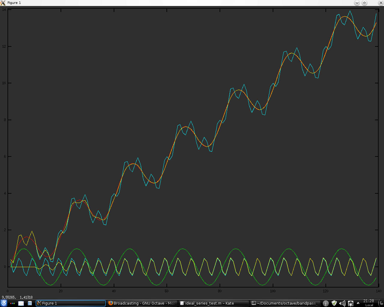
However, the above relates only to random entries in a trend following context, with a trailing stop being set wide enough to "allow the trend to breathe" or "avoid the noise" or other such sayings common in the trend following world. What happens if we tighten the stop? Several 5000 MC runs with a standard deviation stop multiplier of 0.6 shows significant improvement, with the "buy and hold" returns being in the left tail or more than 2 standard deviations away from the average random entry return. To achieve this a fairly tight stop is required, as can be seen below.

Now rather than being a "trend following stop" this could be characterised as a "swing trading stop" where one is trying to get in and out of the market at swing highs and lows. But what if the market is not making swings but is in fact strongly trending as in

which can be achieved by altering a code line thus:

% and create a trending market
trending_market = ((0:1:size(sideways_market,2)-1).*4/period).+sideways_market ;

The same stops as above on this market all show average positive returns, but none so great as to be significantly better than this market's "buy and hold" return of 3.04452. A typical histogram for these tests is

which is quite interesting. The large bar at the right represents those MC runs where the first random position is a long which is not stopped out by the wide stops, hence resulting in a log return for the run of the "buy and hold" log return. The other bars show those MC runs which start with one or more short trades and obviously incur some initial loses prior to the first long trade. Drastically tightening the stop for this market doesn't really help things; the result is still an extreme right hand bar at the "buy and hold" level with a varying left tail.

What all this shows is that the best random entries can do is capture what I called the "bias" in my above quoted thread response, and even doing this well is highly dependent on using a suitable trailing stop; as also mentioned above there are many more opportunities to choose an unsuitable trailing stop. I also suggested that "At a bare minimum, the returns of the tradeable should be detrended to remove this bias before any tests are conducted." The point of this is that by removing the bias it immediately becomes obvious that there is no value in random entries - it will effectively produce the results that the above code gives for the sideways market, shown next.

Standard deviations 2 and 3 are what one might expect - histograms centred around a net log return of zero, standard deviation 4 provides a great opportunity to shoot yourself in the foot by choosing a terrible stop for this market, and standard deviation 1 shows what is possible by choosing a good stop. In fact, by playing around with various values for the stop multiplier I have been able to get values as high as 14 for the net average log return on this market, but such tight stops as these cannot be really be considered trailing stops as they more or less act as take profit stops at the upper and lower levels of this sideways market.

So, what use are random entries? In live trading I believe there is no use whatsoever, but as a "research tool" similar to the approach outlined here there may be some uses. They could be used to set up null hypotheses for statistical testing and benchmarking, or they could be used to see what random looks like in the context of some trading idea. However, the big caveat to this is that if one uses real data how can the randomness in the data, plus any possible non-linear effects of parameter choices, be distinguished from the effects of the "injected randomness" supplied by the random entries? All the forgoing discussion has been based on the clean, simple and predictable data of a fully-known, simulated market, with the intent of illustrating my belief about random entries. When applied portfolio wide on real data, with portfolio heat restrictions, position sizing choices etc. the whole test routine may simply have too many moving parts to draw any useful conclusions about the efficacy of random entries given that statistically speaking, even on the idealised market data used in this post, random entry trend following returns are indistinguishable from buy and hold returns.

Restricted Boltzmann Machine

In an earlier post I said that I would write about Restricted Boltzmann machines and now that I have begun adapting the Geoffrey Hinton course code I have, this is the first post of possibly several on this topic.

Essentially, I am going to use the RBM to conduct unsupervised learning on unlabelled real market data, using some of the indicators I have developed, to extract relevant features to initialise the input to hidden layer weights of my market classifying neural net, and then conduct backpropagation training of this feedforward neural network using the labelled data from my usual, idealised market types.

Readers may well ask, "What's the point of doing this?" Well, taken from my course assignment notes, and edited by me for relevance to this post, we have:-

In the previous assignment we tried to reduce overfitting by learning less (early stopping, fewer hidden units etc.) RBMs, on the other hand, reduce overfitting by learning more: the RBM is being trained unsupervised so it's working to discover a lot of relevant regularity in the input features, and that learning distracts the model from excessively focusing on class labels. This is much more constructive distraction: instead of early stopping the model after a little learning we instead give the model something much more meaningful to do. ...it works great for regularisation, as well as training speed. ... In the previous assignment we did a lot of work selecting the right number of training iterations, the right number of hidden units, and the right weight decay. ... Now we don't need to do that at all, ... the unsupervised training of the RBM provides all the regularisation we need. If we select a decent learning rate, that will be enough, and we'll use lots of hidden units because we're much less worried about overfitting now.

Of course, a picture is worth a thousand words, so below are a 2D and a 3D picture

These two pictures show the weights of the input to hidden layer after only two iterations of RBM training, and effectively represent a "typical" random initialisation of weights prior to backpropagation training. It is from this type of random start that the class labelled data would normally be used to train the NN.

These next two pictures tell a different story

These show weights after 50,000 iterations of RBM training. Quite a difference, and it is from this sort of start that I will now train my market classifier NN using the class labelled data.

Some features are easily seen. Firstly, the six columns on the "left" sides of these pictures result from the cyclic period features in the real data, expressed in binary form, and effectively form the weights that will attach to the NN bias units. Secondly, the "right" side shows the most recent data in the look back window applied to the real market data. The weights here have greater magnitude than those further back, reflecting the fact that shorter periods are more prevalent than longer periods and that, intuitively obvious perhaps, more recent data has greater importance than older data. Finally, the colour mapping shows that across the entire weight matrix the magnitude of the values has been decreased by the RBM training, showing its regularisation effect.

Regime Switching Article

Readers might be interested in this article about Regime Switching, from the IFTA journal, which in intent somewhat mirrors my attempts at market classification via neural net modelling.

Softmax Neural Net Classifier "Half" Complete

Over the last few weeks I have been busy working on the Softmax activation function output neural net classifier and have now reached a point where I have trained it over enough of my usual training data that approximately half of the real data I have would be classified by it, rather than by my previously and incompletely trained "reserve" neural net.

It has taken this long to get this far for a few reasons; the necessity to substantially adapt the code from the Geoff Hinton neural net course and then conducting grid searches over the hyper-parameter space for the "optimum" learning rate, number of neurons in the hidden layer and also incorporating some changes to the features set used as input to the classifier. At this halfway stage I thought I would subject the classifier to the cross validation test of my recent post of 5th December 2012 and the results, which speak for themselves, are shown in the box below.

Random NN
Complete Accuracy percentage: 99.610000

"Acceptable" Mis-classifications percentages 
Predicted = uwr & actual = unr: 0.000000
Predicted = unr & actual = uwr: 0.062000
Predicted = dwr & actual = dnr: 0.008000
Predicted = dnr & actual = dwr: 0.004000
Predicted = uwr & actual = cyc: 0.082000
Predicted = dwr & actual = cyc: 0.004000
Predicted = cyc & actual = uwr: 0.058000
Predicted = cyc & actual = dwr: 0.098000

Dubious, difficult to trade mis-classification percentages 
Predicted = uwr & actual = dwr: 0.000000
Predicted = unr & actual = dwr: 0.000000
Predicted = dwr & actual = uwr: 0.000000
Predicted = dnr & actual = uwr: 0.000000

Completely wrong classifications percentages 
Predicted = unr & actual = dnr: 0.000000
Predicted = dnr & actual = unr: 0.000000

End NN
Complete Accuracy percentage: 98.518000

"Acceptable" Mis-classifications percentages 
Predicted = uwr & actual = unr: 0.002000
Predicted = unr & actual = uwr: 0.310000
Predicted = dwr & actual = dnr: 0.006000
Predicted = dnr & actual = dwr: 0.036000
Predicted = uwr & actual = cyc: 0.272000
Predicted = dwr & actual = cyc: 0.036000
Predicted = cyc & actual = uwr: 0.344000
Predicted = cyc & actual = dwr: 0.210000

Dubious, difficult to trade mis-classification percentages 
Predicted = uwr & actual = dwr: 0.000000
Predicted = unr & actual = dwr: 0.000000
Predicted = dwr & actual = uwr: 0.000000
Predicted = dnr & actual = uwr: 0.000000

Completely wrong classifications percentages 
Predicted = unr & actual = dnr: 0.000000
Predicted = dnr & actual = unr: 0.000000

This classifier has 3 sigmoid logistic neurons in its single hidden layer and during training early stopping was employed. I also tried adding L2 regularization but this didn't really seem to have any appreciable effect, so after a while I dropped this. All in all, I'm very pleased with my efforts and the classifier's performance so far. Over the next few weeks I shall continue with the training and when this is complete I shall post again.

On a related note, I have recently added another blog to the blogroll because I was impressed with a series of posts over the last couple of years concerning that particular blogger's investigations into neural nets for trading, especially the last two posts here and here. The ideas covered in these last two posts ring a bell with my post here, where I first talked about using a neural net as a market classifier based on the work I did in Andrew Ng's course on recognising hand written digits from pixel values. I shall follow this new blogroll addition with interest!